Merge Sort

Divide and conquer algorithms

The two sorting algorithms we've seen so far, selection sort and insertion sort, have worst-case running times of $\Theta(n^2)$. When the size of the input array is large, these algorithms can take a long time to run. In this tutorial and the next one, we'll see two other sorting algorithms, merge sort and quicksort, whose running times are better. In particular, merge sort runs in $\Theta(n \lg n)$ time in all cases, and quicksort runs in $\Theta(n \lg n)$ time in the best case and on average, though its worst-case running time is $\Theta(n^2)$. Here's a table of these four sorting algorithms and their running times:

Algorithm	Worst-case running time	Best-case running time	Average-case running time
Selection sort	$\Theta(n^2)$	$\Theta(n^2)$	$\Theta(n^2)$
Insertion sort	$\Theta(n^2)$	$\Theta(n)$	$\Theta(n^2)$
Merge sort	$\Theta(n \lg n)$	$\Theta(n \lg n)$	$\Theta(n \lg n)$
Quicksort	$\Theta(n^2)$	$\Theta(n \lg n)$	$\Theta(n \lg n)$

Divide-and-conquer

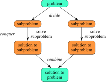
Both merge sort and quicksort employ a common algorithmic paradigm based on recursion. This paradigm, divide-and-conquer, breaks a problem into subproblems that are similar to the original problem, recursively solves the subproblems, and finally combines the solutions to the subproblems to solve the original problem. Because divide-and-conquer solves subproblems recursively, each subproblem must be smaller than the original problem, and there must be a base case for subproblems. You should think of a divide-and-conquer algorithm as having three parts:

1. Divide the problem into a number of subproblems that are smaller instances of the same problem.

2. Conquer the subproblems by solving them recursively. If they are small enough, solve the subproblems as base cases.

3. Combine the solutions to the subproblems into the solution for the original problem.

You can easily remember the steps of a divide-and-conquer algorithm as divide, conquer, combine. Here's how to view one step, assuming that each divide step creates two subproblems (though some divide-and-conquer algorithms create more than two):

If we expand out two more recursive steps, it looks like this:

Because divide-and-conquer creates at least two subproblems, a divide-and-conquer algorithm makes multiple recursive calls.

Overview of merge sort

Because we're using divide-and-conquer to sort, we need to decide what our subproblems are going to look like. The full problem is to sort an entire array. Let's say that a subproblem is to sort a subarray. In particular, we'll think of a subproblem as sorting the subarray starting at index $p$ and going through index $r$. It will be convenient to have a notation for a subarray, so let's say that array[p..r] denotes this subarray of array. Note that this "two-dot" notation is not legal JavaScript; we're using it just to describe the algorithm, rather than a particular implementation of the algorithm in code. In terms of our notation, for an array of $n$ elements, we can say that the original problem is to sort array[0..n-1].Here's how merge sort uses divide-and-conquer:

1. Divide by finding the number $q$ of the position midway between $p$ and $r$. Do this step the same way we found the midpoint in binary search: add $p$and $r$, divide by 2, and round down.
2. Conquer by recursively sorting the subarrays in each of the two subproblems created by the divide step. That is, recursively sort the subarray array[p..q] and recursively sort the subarray array[q+1..r].

3. Combine by merging the two sorted subarrays back into the single sorted subarray array[p..r].

We need a base case. The base case is a subarray containing fewer than two elements, that is, when $p \geq r$, since a subarray with no elements or just one element is already sorted. So we'll divide-conquer-combine only when $p < r$.

Let's see an example. Let's start with array holding [14, 7, 3, 12, 9, 11, 6, 2], so that the first subarray is actually the full array, array[0..7] ($p=0$ and $r=7$). This subarray has at least two elements, and so it's not a base case.

• In the divide step, we compute $q = 3$.
• The conquer step has us sort the two subarrays array[0..3], which contains [14, 7, 3, 12], and array[4..7], which contains [9, 11, 6, 2]. When we come back from the conquer step, each of the two subarrays is sorted: array[0..3] contains [3, 7, 12, 14] and array[4..7] contains [2, 6, 9, 11], so that the full array is [3, 7, 12, 14, 2, 6, 9, 11].

• Finally, the combine step merges the two sorted subarrays in the first half and the second half, producing the final sorted array [2, 3, 6, 7, 9, 11, 12, 14].

How did the subarray array[0..3] become sorted? The same way. It has more than two elements, and so it's not a base case. With $p=0$ and $r=3$, compute $q=1$, recursively sort array[0..1] ([14, 7]) and array[2..3] ([3, 12]), resulting in array[0..3] containing [7, 14, 3, 12], and merge the first half with the second half, producing [3, 7, 12, 14].

How did the subarray array[0..1] become sorted? With $p=0$ and $r=1$, compute $q=0$, recursively sort array[0..0] ([14]) and array[1..1] ([7]), resulting in array[0..1] still containing [14, 7], and merge the first half with the second half, producing [7, 14].

The subarrays array[0..0] and array[1..1] are base cases, since each contains fewer than two elements. Here is how the entire merge sort algorithm unfolds:

Most of the steps in merge sort are simple. You can check for the base case easily. Finding the midpoint $q$ in the divide step is also really easy. You have to make two recursive calls in the conquer step. It's the combine step, where you have to merge two sorted subarrays, where the real work happens.

In the next challenge, you'll focus on implementing the overall merge sort algorithm, to make sure you understand how to divide and conquer recursively. After you've done that, we'll dive deeper into how to merge two sorted subarrays efficiently and you'll implement that in the later challenge.

// Takes in an array that has two sorted subarrays,
//  from [p..q] and [q+1..r], and merges the array
var merge = function(array, p, q, r) {
    var lowHalf = [], 
        highHalf = [], 
        k = p, d, e;
    // get everything on the left side
    for (d = 0; k <= q; d++, k++) {
        lowHalf[d] = array[k];
    }
    // get everything on the right side
    for (e = 0; k <= r; e++, k++) {
        highHalf[e] = array[k];
    }
    // switch elements if needed
    k = p;
    for (e = d = 0; d < lowHalf.length && e < highHalf.length;) {
        if (lowHalf[d] < highHalf[e]) {
            array[k] = lowHalf[d];
            d++;
        } else {
            array[k] = highHalf[e];
            e++;
        }
        k++;
    }
    // left side
    for (; d < lowHalf.length;) {
        array[k] = lowHalf[d];
        d++;
        k++;
    }
    // right side
    for (; e < highHalf.length;) {
        array[k] = highHalf[e];
        e++;
        k++;
    }
};

// Takes in an array and recursively merge sorts it
var mergeSort = function(array, p, r) {
    if (r > p) {
        var q = floor((r-p)/2) + p;
        mergeSort(array, p, q); 
        mergeSort(array, q+1, r);
        merge(array, p, q, r);
    }
};

var array = [14, 7, 3, 12, 9, 11, 6, 2];
mergeSort(array, 0, array.length-1);
println("Array after sorting: " + array);
// Program.assertEqual(array, [2, 3, 6, 7, 9, 11, 12, 14]);

Linear-time merging

The remaining piece of merge sort is the merge function, which merges two adjacent sorted subarrays, array[p..q] and array[q+1..r] into a single sorted subarray in array[p..r]. We'll see how to construct this function so that it's as efficient as possible. Let's say that the two subarrays have a total of $n$ elements. We have to examine each of the elements in order to merge them together, and so the best we can hope for would be a merging time of $\Theta(n)$. Indeed, we'll see how to merge a total of $n$ elements in $\Theta(n)$ time.

In order to merge the sorted subarrays array[p..q] and array[q+1..r] and have the result in array[p..r], we first need to make temporary arrays and copy array[p..q] and array[q+1..r] into these temporary arrays. We can't write over the positions in array[p..r] until we have the elements originally in array[p..q] and array[q+1..r] safely copied.

The first order of business in the merge function, therefore, is to allocate two temporary arrays, lowHalf and highHalf, to copy all the elements in array[p..q] into lowHalf, and to copy all the elements in array[q+1..r]into highHalf. How big should lowHalf be? The subarray array[p..q]contains $q-p+1$ elements. How about highHalf? The subarray array[q+1..r] contains $r-q$ elements. (In JavaScript, we don't have to give the size of an array when we create it, but since we do have to do that in many other programming languages, we often consider it when describing an algorithm.)

In our example array [14, 7, 3, 12, 9, 11, 6, 2], here's what things look like after we've recursively sorted array[0..3] and array[4..7] (so that $p=0$, $q=3$, and $r=7$) and copied these subarrays into lowHalf and highHalf:

The numbers in array are grayed out to indicate that although these array positions contain values, the "real" values are now in lowHalf and highHalf. We may overwrite the grayed numbers at will.

Next, we merge the two sorted subarrays, now in lowHalf and highHalf, back into array[p..r]. We should put the smallest value in either of the two subarrays into array[p]. Where might this smallest value reside? Because the subarrays are sorted, the smallest value must be in one of just two places: either lowHalf[0] or highHalf[0]. (It's possible that the same value is in both places, and then we can call either one the smallest value.) With just one comparison, we can determine whether to copy lowHalf[0] or highHalf[0]into array[p]. In our example, highHalf[0] was smaller. Let's also establish three variables to index into the arrays:

• i indexes the next element of lowHalf that we have not copied back into array. Initially, i is 0.

• j indexes the next element of highHalf that we have not copied back into array. Initially, j is 0.

• k indexes the next location in array that we copy into. Initially, k equals p.

After we copy from lowHalf or highHalf into array, we must increment (add 1 to) k so that we copy the next smallest element into the next position of array. We also have to increment i if we copied from lowHalf, or increment j if we copied from highHalf. So here are the arrays before and after the first element is copied back into array:

We've grayed out highHalf[0] to indicate that it no longer contains a value that we're going to consider. The un-merged part of the highHalf array starts at index j, which is now 1. The value in array[p] is no longer grayed out, because we copied a "real" value into it.

Where must the next value to copy back into array reside? It's either first untaken element in lowHalf (lowHalf[0]) or the first untaken element in highHalf (highHalf[1]). With one comparison, we determine that lowHalf[0] is smaller, and so we copy it into array[k] and increment k and i:

Next, we compare lowHalf[1] and highHalf[1], determining that we should copy highHalf[1] into array[k]. We then increment k and j:

Keep going, always comparing lowHalf[i] and highHalf[j], copying the smaller of the two into array[k], and incrementing either i or j:

Eventually, either all of lowHalf or all of highHalf is copied back into array. In this example, all of highHalf is copied back before the last few elements of lowHalf. We finish up by just copying the remaining untaken elements in either lowHalf or highHalf:

We claimed that merging $n$ elements takes $\Theta(n)$ time, and therefore the running time of merging is linear in the subarray size. Let's see why this is true. We saw three parts to merging:

1. Copy each element in array[p..r] into either lowHalf or highHalf.

2. As long as some elements are untaken in both lowHalf and highHalf, compare the first two untaken elements and copy the smaller one back into array.

3. Once either lowHalf or highHalf has had all its elements copied back into array, copy each remaining untaken element from the other temporary array back into array.

How many lines of code do we need to execute for each of these steps? It's a constant number per element. Each element is copied from array into either lowHalf or highHalf exactly one time in step 1. Each comparison in step 2 takes constant time, since it compares just two elements, and each element "wins" a comparison at most one time. Each element is copied back into arrayexactly one time in steps 2 and 3 combined. Since we execute each line of code a constant number of times per element and we assume that the subarray array[p..q] contains $n$ elements, the running time for merging is indeed $\Theta(n)$.

Analysis of merge sort

Given that the merge function runs in $\Theta(n)$ time when merging $n$ elements, how do we get to showing that mergeSort runs in $\Theta(n \log_2 n)$ time? We start by thinking about the three parts of divide-and-conquer and how to account for their running times. We assume that we're sorting a total of $n$ elements in the entire array.

1. The divide step takes constant time, regardless of the subarray size. After all, the divide step just computes the midpoint $q$ of the indices $p$ and $r$. Recall that in big-Θ notation, we indicate constant time by $\Theta(1)$.
2. The conquer step, where we recursively sort two subarrays of approximately $n/2$ elements each, takes some amount of time, but we'll account for that time when we consider the subproblems.
3. The combine step merges a total of $n$ elements, taking $\Theta(n)$time.

If we think about the divide and combine steps together, the $\Theta(1)$ running time for the divide step is a low-order term when compared with the $\Theta(n)$running time of the combine step. So let's think of the divide and combine steps together as taking $\Theta(n)$ time. To make things more concrete, let's say that the divide and combine steps together take $cn$ time for some constant $c$.

To keep things reasonably simple, let's assume that if $n>1$, then $n$ is always even, so that when we need to think about $n/2$, it's an integer. (Accounting for the case in which $n$ is odd doesn't change the result in terms of big-Θ notation.) So now we can think of the running time of mergeSort on an $n$-element subarray as being the sum of twice the running time of mergeSort on an ($n/2$)-element subarray (for the conquer step) plus $cn$ (for the divide and combine steps—really for just the merging).

Now we have to figure out the running time of two recursive calls on $n/2$ elements. Each of these two recursive calls takes twice of the running time of mergeSort on an $(n/4)$-element subarray (because we have to halve $n/2$) plus $cn/2$ to merge. We have two subproblems of size $n/2$, and each takes $cn/2$ time to merge, and so the total time we spend merging for subproblems of size $n/2$ is $2\cdot cn/2 = cn$.

Let's draw out the merging times in a "tree":

Computer scientists draw trees upside-down from how actual trees grow. A tree is a graph with no cycles (paths that start and end at the same place). Convention is to call the vertices in a tree its nodes. The root node is on top; here, the root is labeled with the $n$ subarray size for the original $n$-element array. Below the root are two child nodes, each labeled $n/2$ to represent the subarray sizes for the two subproblems of size $n/2$.

Each of the subproblems of size $n/2$ recursively sorts two subarrays of size $(n/2)/2$, or $n/4$. Because there are two subproblems of size $n/2$, there are four subproblems of size $n/4$. Each of these four subproblems merges a total of $n/4$ elements, and so the merging time for each of the four subproblems is $cn/4$. Summed up over the four subproblems, we see that the total merging time for all subproblems of size $n/4$ is $4 \cdot cn/4 = cn$:

What do you think would happen for the subproblems of size $n/8$? There will be eight of them, and the merging time for each will be $cn/8$, for a total merging time of $8 \cdot cn/8 = cn$:

As the subproblems get smaller, the number of subproblems doubles at each "level" of the recursion, but the merging time halves. The doubling and halving cancel each other out, and so the total merging time is $cn$ at each level of recursion. Eventually, we get down to subproblems of size 1: the base case. We have to spend $\Theta(1)$ time to sort subarrays of size 1, because we have to test whether $p < r$, and this test takes time. How many subarrays of size 1 are there? Since we started with $n$ elements, there must be $n$ of them. Since each base case takes $\Theta(1)$ time, let's say that altogether, the base cases take $cn$ -time:

Now we know how long merging takes for each subproblem size. The total time for mergeSort is the sum of the merging times for all the levels. If there are $l$ levels in the tree, then the total merging time is $l \cdot cn$. So what is $l$? We start with subproblems of size $n$ and repeatedly halve until we get down to subproblems of size 1. We saw this characteristic when we analyzed binary search, and the answer is $l = \log_2 n + 1$. For example, if $n=8$, then $\log_2 n + 1 = 4$, and sure enough, the tree has four levels: $n = 8, 4, 2, 1$. The total time for mergeSort, then, is $cn (\log_2 n + 1)$. When we use big-Θ notation to describe this running time, we can discard the low-order term $(+1)$ and the constant coefficient $(c)$, giving us a running time of $\Theta(n \log_2 n)$, as promised.

One other thing about merge sort is worth noting. During merging, it makes a copy of the entire array being sorted, with one half in lowHalf and the other half in highHalf. Because it copies more than a constant number of elements at some time, we say that merge sort does not work in place. By contrast, both selection sort and insertion sort do work in place, since they never make a copy of more than a constant number of array elements at any one time. Computer scientists like to consider whether an algorithm works in place, because there are some systems where space is at a premium, and thus in-place algorithms are preferred.