What is a CapsNet or Capsule Network?

What is a Capsule Network? What is a Capsule? Is CapsNet better than a Convolutional Neural Network (CNN)? In this article I will talk about all the above questions about CapsNet or Capsule Network released by Hinton.

Note: This article is not about pharmaceutical capsules. It is about Capsules in Neural Networks or Machine Learning world.

There is an expectation from you as a reader. You need to be aware of CNNs. If not, I would like you to go through this article on Hackernoon. Next I will run through a small recap of relevant points of CNN. That way you can easily grab on to the comparison done below. So without further ado lets dive in.

CNN are essentially a system where we stack a lot of neurons together. These networks have been proven to be exceptionally great at handling image classification problems. It would be hard to have a neural network map out all the pixels of an image since it‘s computationally really expensive. So convolutional is a method which helps you simplify the computation to a great extent without losing the essence of the data. Convolution is basically a lot of matrix multiplication and summation of those results.image 1.0: Convolutional Neural Network

After an image is fed to the network, a set of kernels or filters scan it and perform the convolution operation. This leads to creation of feature maps inside the network. These features next pass via activation layer and pooling layers in succession and then based on the number of layers in the network this continues. Activation layers are required to induce a sense of non linearityin the network (eg: ReLU). Pooling (eg: max pooling) helps in reducing the training time. The idea of pooling is that it creates “summaries” of each sub-region. It also gives you a little bit of positional and translational invariance in object detection. At the end of the network it will pass via a classifier like softmax classifier which will give us a class. Training happens based on back propagation of error matched against some labelled data. Non linearity also helps in solving the vanishing gradient in this step.

What is the problem with CNNs?

CNNs perform exceptionally great when they are classifying images which are very close to the data set. If the images have rotation, tilt or any other different orientation then CNNs have poor performance. This problem was solved by adding different variations of the same image during training. In CNN each layer understands an image at a much more granular level. Lets understand this with an example. If you are trying to classify ships and horses. The innermost layer or the 1st layer understands the small curves and edges. The 2nd layer might understand the straight lines or the smaller shapes, like the mast of a ship or the curvature of the entire tail. Higher up layers start understanding more complex shapes like the entire tail or the ship hull. Final layers try to see a more holistic picture like the entire ship or the entire horse. We use pooling after each layer to make it compute in reasonable time frames. But in essence it also loses out the positional data.image 2.0: Disfiguration transformation

Pooling helps in creating the positional invariance. Otherwise CNNs would fit only for images or data which are very close to the training set. This invariance also leads to triggering false positive for images which have the components of a ship but not in the correct order. So the system can trigger the right to match with the left in the above image. You as an observer clearly see the difference. The pooling layer also adds this sort of invariance.image 2.1 Proportional transformation

This was never the intention of pooling layer. What the pooling was supposed to do is to introduce positional, orientational, proportional invariances. But the method we use to get this uses is very crude. In reality it adds all sorts of positional invariance. Thus leading to the dilemma of detecting right ship in image 2.0 as a correct ship. What we needed was not invariance but equivariance. Invariance makes a CNN tolerant to small changes in the viewpoint. Equivariance makes a CNN understand the rotation or proportion change and adapt itself accordingly so that the spatial positioning inside an image is not lost. A ship will still be a smaller ship but the CNN will reduce its size to detect that. This leads us to the recent advancement of Capsule Networks.

What is a Capsule Network?

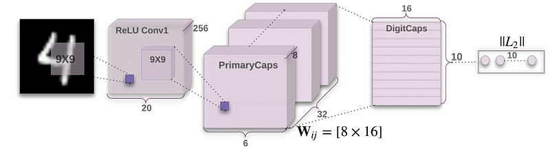
Every few days there is an advancement in the field of Neural Networks. Some brilliant minds are working on this field. You can pretty much assume every paper on this topic is almost ground breaking or path changing. Sara Sabour, Nicholas Frost and Geoffrey Hinton released a paper titled “Dynamic Routing Between Capsules” 4 days back. Now when one of the Godfathers of Deep Learning “Geoffrey Hinton” is releasing a paper it is bound to be ground breaking. The entire Deep Learning community is going crazy on this paper as you read this article. So this paper talks about Capsules, CapsNet and a run on MNIST. MNIST is a database of tagged handwritten digit images. Results are showing a significant increase in performance in case of overlapped digits. The paper compares to the current state-of-the-art CNNs. In this paper the authors project that human brain have modules called “capsules”. These capsules are particularly good at handling different types of visual stimulus and encoding things like pose (position, size, orientation), deformation, velocity, albedo, hue, texture etc. The brain must have a mechanism for “routing” low level visual information to what it believes is the best capsule for handling it.image 3.0: CapsNet Architecture

Capsule is a nested set of neural layers. So in a regular neural network you keep on adding more layers. In CapsNet you would add more layers inside a single layer. Or in other words nest a neural layer inside another. The state of the neurons inside a capsule capture the above properties of one entity inside an image. A capsule outputs a vector to represent the existence of the entity. The orientation of the vector represents the properties of the entity. The vector is sent to all possible parents in the neural network. For each possible parent a capsule can find a prediction vector. Prediction vector is calculated based on multiplying it’s own weight and a weight matrix. Whichever parent has the largest scalar prediction vector product, increases the capsule bond. Rest of the parents decrease their bond. This routing by agreement method is superior than the current mechanism like max-pooling. Max pooling routes based on the strongest feature detected in the lower layer. Apart from dynamic routing, CapsNet talks about adding squashing to a capsule. Squashing is a non-linearity. So instead of adding squashing to each layer like how you do in CNN, you add the squashing to a nested set of layers. So the squashing function gets applied to the vector output of each capsule.image 3.1: Novel Squashing Function

The paper introduces a new squashing function. You can see it in image 3.1. ReLU or similar non linearity functions work well with single neurons. But the paper found that this squashing function works best with capsules. This tries to squash the length of output vector of a capsule. It squashes to 0 if it is a small vector and tries to limit the output vector to 1 if the vector is long. The dynamic routing adds some extra computation cost. But it definitely gives added advantage.

Now we need to realise that this paper is almost brand new and the concept of capsules is not throughly tested. It works on MNIST data but it still needs to be proven against much larger dataset across a variety of classes. There are already (within 4 days) updates on this paper who raise the following concerns:

1. It uses the length of the pose vector to represent the probability that the entity represented by a capsule is present. To keep the length less than 1 requires an unprincipled non-linearity that prevents there from being any sensible objective function that is minimized by the iterative routing procedure.

2. It uses the cosine of the angle between two pose vectors to measure their agreement for routing. Unlike the log variance of a Gaussian cluster, the cosine is not good at distinguishing between quite good agreement and very good agreement.

3. It uses a vector of length n rather than a matrix with n elements to represent a pose, so its transformation matrices have n 2 parameters rather than just n.

The current implementation of capsules has scope for improvement. But we should also keep in mind that the Hinton paper in the first place only says:

The aim of this paper is not to explore this whole space but to simply show that one fairly straightforward implementation works well and that dynamic routing helps.

So that’s a lot of theory. Lets have some fun and build a CapsNet. I will take you through some code to setup a basic CapsNet for MNIST data. I will comment inside the code so you can follow through line by line and get an understanding of how it works. I will take you through two important pieces in the code. Rest you can go to the repo, fork it and start working on it:

# It only has two dependencies numpy and tensorflow
import numpy as np
import tensorflow as tf

from config import cfg


# Class defining a Convolutional Capsule
# consisting of multiple neuron layers
#
class CapsConv(object):
    ''' Capsule layer.
    Args:
        input: A 4-D tensor.
        num_units: integer, the length of the output vector of a capsule.
        with_routing: boolean, this capsule is routing with the
                      lower-level layer capsule.
        num_outputs: the number of capsule in this layer.
    Returns:
        A 4-D tensor.
    '''
    def __init__(self, num_units, with_routing=True):
        self.num_units = num_units
        self.with_routing = with_routing

    def __call__(self, input, num_outputs, kernel_size=None, stride=None):
        self.num_outputs = num_outputs
        self.kernel_size = kernel_size
        self.stride = stride

        if not self.with_routing:
            # the PrimaryCaps layer
            # input: [batch_size, 20, 20, 256]
            assert input.get_shape() == [cfg.batch_size, 20, 20, 256]

            capsules = []
            for i in range(self.num_units):
                # each capsule i: [batch_size, 6, 6, 32]
                with tf.variable_scope('ConvUnit_' + str(i)):
                    caps_i = tf.contrib.layers.conv2d(input,
                                                      self.num_outputs,
                                                      self.kernel_size,
                                                      self.stride,
                                                      padding="VALID")
                    caps_i = tf.reshape(caps_i, shape=(cfg.batch_size, -1, 1, 1))
                    capsules.append(caps_i)

            assert capsules[0].get_shape() == [cfg.batch_size, 1152, 1, 1]

            # [batch_size, 1152, 8, 1]
            capsules = tf.concat(capsules, axis=2)
            capsules = squash(capsules)
            assert capsules.get_shape() == [cfg.batch_size, 1152, 8, 1]

        else:
            # the DigitCaps layer
            # Reshape the input into shape [batch_size, 1152, 8, 1]
            self.input = tf.reshape(input, shape=(cfg.batch_size, 1152, 8, 1))

            # b_IJ: [1, num_caps_l, num_caps_l_plus_1, 1]
            b_IJ = tf.zeros(shape=[1, 1152, 10, 1], dtype=np.float32)
            capsules = []
            for j in range(self.num_outputs):
                with tf.variable_scope('caps_' + str(j)):
                    caps_j, b_IJ = capsule(input, b_IJ, j)
                    capsules.append(caps_j)

            # Return a tensor with shape [batch_size, 10, 16, 1]
            capsules = tf.concat(capsules, axis=1)
            assert capsules.get_shape() == [cfg.batch_size, 10, 16, 1]

        return(capsules)


def capsule(input, b_IJ, idx_j):
    ''' The routing algorithm for one capsule in the layer l+1.
    Args:
        input: A Tensor with [batch_size, num_caps_l=1152, length(u_i)=8, 1]
               shape, num_caps_l meaning the number of capsule in the layer l.
    Returns:
        A Tensor of shape [batch_size, 1, length(v_j)=16, 1] representing the
        vector output `v_j` of capsule j in the layer l+1
    Notes:
        u_i represents the vector output of capsule i in the layer l, and
        v_j the vector output of capsule j in the layer l+1.
     '''

    with tf.variable_scope('routing'):
        w_initializer = np.random.normal(size=[1, 1152, 8, 16], scale=0.01)
        W_Ij = tf.Variable(w_initializer, dtype=tf.float32)
        # repeat W_Ij with batch_size times to shape [batch_size, 1152, 8, 16]
        W_Ij = tf.tile(W_Ij, [cfg.batch_size, 1, 1, 1])

        # calc u_hat
        # [8, 16].T x [8, 1] => [16, 1] => [batch_size, 1152, 16, 1]
        u_hat = tf.matmul(W_Ij, input, transpose_a=True)
        assert u_hat.get_shape() == [cfg.batch_size, 1152, 16, 1]

        shape = b_IJ.get_shape().as_list()
        size_splits = [idx_j, 1, shape[2] - idx_j - 1]
        for r_iter in range(cfg.iter_routing):
            # line 4:
            # [1, 1152, 10, 1]
            c_IJ = tf.nn.softmax(b_IJ, dim=2)
            assert c_IJ.get_shape() == [1, 1152, 10, 1]

            # line 5:
            # weighting u_hat with c_I in the third dim,
            # then sum in the second dim, resulting in [batch_size, 1, 16, 1]
            b_Il, b_Ij, b_Ir = tf.split(b_IJ, size_splits, axis=2)
            c_Il, c_Ij, b_Ir = tf.split(c_IJ, size_splits, axis=2)
            assert c_Ij.get_shape() == [1, 1152, 1, 1]

            s_j = tf.multiply(c_Ij, u_hat)
            s_j = tf.reduce_sum(tf.multiply(c_Ij, u_hat),
                                axis=1, keep_dims=True)
            assert s_j.get_shape() == [cfg.batch_size, 1, 16, 1]

            # line 6:
            # squash using Eq.1, resulting in [batch_size, 1, 16, 1]
            v_j = squash(s_j)
            assert s_j.get_shape() == [cfg.batch_size, 1, 16, 1]

            # line 7:
            # tile v_j from [batch_size ,1, 16, 1] to [batch_size, 1152, 16, 1]
            # [16, 1].T x [16, 1] => [1, 1], then reduce mean in the
            # batch_size dim, resulting in [1, 1152, 1, 1]
            v_j_tiled = tf.tile(v_j, [1, 1152, 1, 1])
            u_produce_v = tf.matmul(u_hat, v_j_tiled, transpose_a=True)
            assert u_produce_v.get_shape() == [cfg.batch_size, 1152, 1, 1]
            b_Ij += tf.reduce_sum(u_produce_v, axis=0, keep_dims=True)
            b_IJ = tf.concat([b_Il, b_Ij, b_Ir], axis=2)

        return(v_j, b_IJ)


def squash(vector):
    '''Squashing function.
    Args:
        vector: A 4-D tensor with shape [batch_size, num_caps, vec_len, 1],
    Returns:
        A 4-D tensor with the same shape as vector but
        squashed in 3rd and 4th dimensions.
    '''
    vec_abs = tf.sqrt(tf.reduce_sum(tf.square(vector)))  # a scalar
    scalar_factor = tf.square(vec_abs) / (1 + tf.square(vec_abs))
    vec_squashed = scalar_factor * tf.divide(vector, vec_abs)  # element-wise
    return(vec_squashed)

The above is the entire Capsule layer. This is now stacked to created a Capsule Network. Code for CapsNet is below:

import tensorflow as tf

from config import cfg
from utils import get_batch_data
from capsLayer import CapsConv


class CapsNet(object):
    def __init__(self, is_training=True):
        self.graph = tf.Graph()
        with self.graph.as_default():
            if is_training:
                self.X, self.Y = get_batch_data()

                self.build_arch()
                self.loss()

                # t_vars = tf.trainable_variables()
                self.optimizer = tf.train.AdamOptimizer()
                self.global_step = tf.Variable(0, name='global_step', trainable=False)
                self.train_op = self.optimizer.minimize(self.total_loss, global_step=self.global_step)  # var_list=t_vars)
            else:
                self.X = tf.placeholder(tf.float32,
                                        shape=(cfg.batch_size, 28, 28, 1))
                self.build_arch()

        tf.logging.info('Seting up the main structure')

    def build_arch(self):
        with tf.variable_scope('Conv1_layer'):
            # Conv1, [batch_size, 20, 20, 256]
            conv1 = tf.contrib.layers.conv2d(self.X, num_outputs=256,
                                             kernel_size=9, stride=1,
                                             padding='VALID')
            assert conv1.get_shape() == [cfg.batch_size, 20, 20, 256]

        # TODO: Rewrite the 'CapsConv' class as a function, the capsLay
        # function should be encapsulated into tow function, one like conv2d
        # and another is fully_connected in Tensorflow.
        # Primary Capsules, [batch_size, 1152, 8, 1]
        with tf.variable_scope('PrimaryCaps_layer'):
            primaryCaps = CapsConv(num_units=8, with_routing=False)
            caps1 = primaryCaps(conv1, num_outputs=32, kernel_size=9, stride=2)
            assert caps1.get_shape() == [cfg.batch_size, 1152, 8, 1]

        # DigitCaps layer, [batch_size, 10, 16, 1]
        with tf.variable_scope('DigitCaps_layer'):
            digitCaps = CapsConv(num_units=16, with_routing=True)
            self.caps2 = digitCaps(caps1, num_outputs=10)

        # Decoder structure in Fig. 2
        # 1. Do masking, how:
        with tf.variable_scope('Masking'):
            # a). calc ||v_c||, then do softmax(||v_c||)
            # [batch_size, 10, 16, 1] => [batch_size, 10, 1, 1]
            self.v_length = tf.sqrt(tf.reduce_sum(tf.square(self.caps2),
                                                  axis=2, keep_dims=True))
            self.softmax_v = tf.nn.softmax(self.v_length, dim=1)
            assert self.softmax_v.get_shape() == [cfg.batch_size, 10, 1, 1]

            # b). pick out the index of max softmax val of the 10 caps
            # [batch_size, 10, 1, 1] => [batch_size] (index)
            argmax_idx = tf.argmax(self.softmax_v, axis=1, output_type=tf.int32)
            assert argmax_idx.get_shape() == [cfg.batch_size, 1, 1]

            # c). indexing
            # It's not easy to understand the indexing process with argmax_idx
            # as we are 3-dim animal
            masked_v = []
            argmax_idx = tf.reshape(argmax_idx, shape=(cfg.batch_size, ))
            for batch_size in range(cfg.batch_size):
                v = self.caps2[batch_size][argmax_idx[batch_size], :]
                masked_v.append(tf.reshape(v, shape=(1, 1, 16, 1)))

            self.masked_v = tf.concat(masked_v, axis=0)
            assert self.masked_v.get_shape() == [cfg.batch_size, 1, 16, 1]

        # 2. Reconstructe the MNIST images with 3 FC layers
        # [batch_size, 1, 16, 1] => [batch_size, 16] => [batch_size, 512]
        with tf.variable_scope('Decoder'):
            vector_j = tf.reshape(self.masked_v, shape=(cfg.batch_size, -1))
            fc1 = tf.contrib.layers.fully_connected(vector_j, num_outputs=512)
            assert fc1.get_shape() == [cfg.batch_size, 512]
            fc2 = tf.contrib.layers.fully_connected(fc1, num_outputs=1024)
            assert fc2.get_shape() == [cfg.batch_size, 1024]
            self.decoded = tf.contrib.layers.fully_connected(fc2, num_outputs=784, activation_fn=tf.sigmoid)

    def loss(self):
        # 1. The margin loss

        # [batch_size, 10, 1, 1]
        # max_l = max(0, m_plus-||v_c||)^2
        max_l = tf.square(tf.maximum(0., cfg.m_plus - self.v_length))
        # max_r = max(0, ||v_c||-m_minus)^2
        max_r = tf.square(tf.maximum(0., self.v_length - cfg.m_minus))
        assert max_l.get_shape() == [cfg.batch_size, 10, 1, 1]

        # reshape: [batch_size, 10, 1, 1] => [batch_size, 10]
        max_l = tf.reshape(max_l, shape=(cfg.batch_size, -1))
        max_r = tf.reshape(max_r, shape=(cfg.batch_size, -1))

        # calc T_c: [batch_size, 10]
        # T_c = Y, is my understanding correct? Try it.
        T_c = self.Y
        # [batch_size, 10], element-wise multiply
        L_c = T_c * max_l + cfg.lambda_val * (1 - T_c) * max_r

        self.margin_loss = tf.reduce_mean(tf.reduce_sum(L_c, axis=1))

        # 2. The reconstruction loss
        orgin = tf.reshape(self.X, shape=(cfg.batch_size, -1))
        squared = tf.square(self.decoded - orgin)
        self.reconstruction_err = tf.reduce_mean(squared)

        # 3. Total loss
        self.total_loss = self.margin_loss + 0.0005 * self.reconstruction_err

        # Summary
        tf.summary.scalar('margin_loss', self.margin_loss)
        tf.summary.scalar('reconstruction_loss', self.reconstruction_err)
        tf.summary.scalar('total_loss', self.total_loss)
        recon_img = tf.reshape(self.decoded, shape=(cfg.batch_size, 28, 28, 1))
        tf.summary.image('reconstruction_img', recon_img)
        self.merged_sum = tf.summary.merge_all()

The entire code along with the training and evaluation module is present here. It’s under Apache 2.0 License. You can use it freely. I want to give credits for the code to naturomics.

Summary

So we went through what is a CapsNet and how they are built. We tried to understand that capsules are nothing but nested neural layers on a high level. We also looked at how a CapsNet delivers rotational and other invariances. It does that being equivariant to the spatial setup of the each entity inside an image. I am sure there are still questions to be answered. Capsules and their best implementation is probably the biggest question. But this post is an initial push in trying to throw some light on the topic. If you have any queries please do share them. I will answer them to the best of my knowledge.