> For the complete documentation index, see [llms.txt](https://stephanosterburg.gitbook.io/scrapbook/llms.txt). Markdown versions of documentation pages are available by appending `.md` to page URLs; this page is available as [Markdown](https://stephanosterburg.gitbook.io/scrapbook/coding/intro-to-tensorflow-for-ai-ml-and-dl/an-overview-of-resnet-and-its-variants.md).
# An Overview of ResNet and its Variants
After the celebrated victory of AlexNet \[1] at the LSVRC2012 classification contest, deep Residual Network \[2] was arguably the most groundbreaking work in the computer vision/deep learning community in the last few years. ResNet makes it possible to train up to hundreds or even thousands of layers and still achieves compelling performance.
Taking advantage of its powerful representational ability, the performance of many computer vision applications other than image classification have been boosted, such as object detection and face recognition.
Since ResNet blew people’s mind in 2015, many in the research community have dived into the secrets of its success, many refinements have been made in the architecture. This article is divided into two parts, in the first part I am going to give a little bit of background knowledge for those who are unfamiliar with ResNet, in the second I will review some of the papers I read recently regarding different variants and interpretations of the ResNet architecture.
#### Revisiting ResNet
According to the universal approximation theorem, given enough capacity, we know that a feedforward network with a single layer is sufficient to represent any function. However, the layer might be massive and the network is prone to overfitting the data. Therefore, there is a common trend in the research community that our network architecture needs to go deeper.
Since AlexNet, the state-of-the-art CNN architecture is going deeper and deeper. While AlexNet had only 5 convolutional layers, the VGG network \[3] and GoogleNet (also codenamed Inception\_v1) \[4] had 19 and 22 layers respectively.
However, increasing network depth does not work by simply stacking layers together. Deep networks are hard to train because of the notorious vanishing gradient problem — as the gradient is back-propagated to earlier layers, repeated multiplication may make the gradient infinitively small. As a result, as the network goes deeper, its performance gets saturated or even starts degrading rapidly.increasing network depth leads to worse performance

Before ResNet, there had been several ways to deal the vanishing gradient issue, for instance, \[4] adds an auxiliary loss in a middle layer as extra supervision, but none seemed to really tackle the problem once and for all.
The core idea of ResNet is introducing a so-called “identity shortcut connection” that skips one or more layers, as shown in the following figure:a residual blockthe ResNet architecture
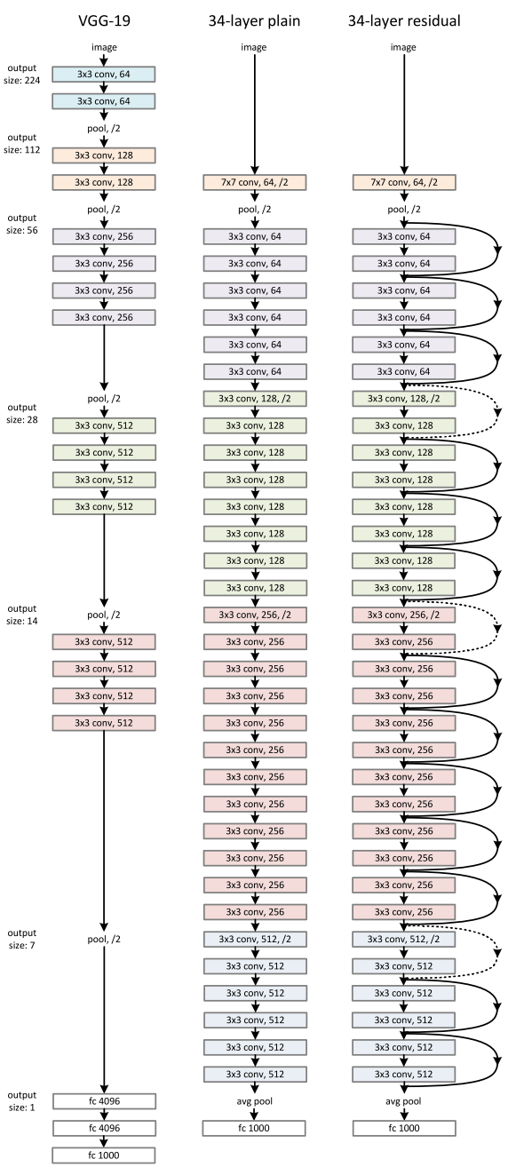

The authors of \[2] argue that stacking layers shouldn’t degrade the network performance, because we could simply stack identity mappings (layer that doesn’t do anything) upon the current network, and the resulting architecture would perform the same. This indicates that the deeper model should not produce a training error higher than its shallower counterparts. They hypothesize that letting the stacked layers fit a residual mapping is easier than letting them directly fit the desired underlaying mapping. And the residual block above explicitly allows it to do precisely that.
As a matter of fact, ResNet was not the first to make use of shortcut connections, Highway Network \[5] introduced gated shortcut connections. These parameterized gates control how much information is allowed to flow across the shortcut. Similar idea can be found in the Long Term Short Memory (LSTM) \[6] cell, in which there is a parameterized forget gate that controls how much information will flow to the next time step. Therefore, ResNet can be thought of as a special case of Highway Network.
However, experiments show that Highway Network performs no better than ResNet, which is kind of strange because the solution space of Highway Network contains ResNet, therefore it should perform at least as good as ResNet. This suggests that it is more important to keep these “gradient highways” clear than to go for larger solution space.
Following this intuition, the authors of \[2] refined the residual block and proposed a pre-activation variant of residual block \[7], in which the gradients can flow through the shortcut connections to any other earlier layer unimpededly. In fact, using the original residual block in \[2], training a 1202-layer ResNet resulted in worse performance than its 110-layer counterpart.variants of residual blocks

The authors of \[7] demonstrated with experiments that they can now train a 1001-layer deep ResNet to outperform its shallower counterparts. Because of its compelling results, ResNet quickly became one of the most popular architectures in various computer vision tasks.
#### Recent Variants and Interpretations of ResNet
As ResNet gains more and more popularity in the research community, its architecture is getting studied heavily. In this section, I will first introduce several new architectures based on ResNet, then introduce a paper that provides an interpretation of treating ResNet as an ensemble of many smaller networks.
**ResNeXt**
Xie et al. \[8] proposed a variant of ResNet that is codenamed ResNeXt with the following building block:left: a building block of \[2], right: a building block of ResNeXt with cardinality = 32

This may look familiar to you as it is very similar to the Inception module of \[4], they both follow the split-transform-merge paradigm, except in this variant, the outputs of different paths are merged by adding them together, while in \[4] they are depth-concatenated. Another difference is that in \[4], each path is different (1x1, 3x3 and 5x5 convolution) from each other, while in this architecture, all paths share the same topology.
The authors introduced a hyper-parameter called cardinality — the number of independent paths, to provide a new way of adjusting the model capacity. Experiments show that accuracy can be gained more efficiently by increasing the cardinality than by going deeper or wider. The authors state that compared to Inception, this novel architecture is easier to adapt to new datasets/tasks, as it has a simple paradigm and only one hyper-parameter to be adjusted, while Inception has many hyper-parameters (like the kernel size of the convolutional layer of each path) to tune.
This novel building block has three equivalent form as follows:

In practice, the “split-transform-merge” is usually done by pointwise grouped convolutional layer, which divides its input into groups of feature maps and perform normal convolution respectively, their outputs are depth-concatenated and then fed to a 1x1 convolutional layer.
**Densely Connected CNN**
Huang et al. \[9] proposed a novel architecture called DenseNet that further exploits the effects of shortcut connections — it connects all layers directly with each other. In this novel architecture, the input of each layer consists of the feature maps of all earlier layer, and its output is passed to each subsequent layer. The feature maps are aggregated with depth-concatenation.

Other than tackling the vanishing gradients problem, the authors of \[8] argue that this architecture also encourages feature reuse, making the network highly parameter-efficient. One simple interpretation of this is that, in \[2]\[7], the output of the identity mapping was added to the next block, which might impede information flow if the feature maps of two layers have very different distributions. Therefore, concatenating feature maps can preserve them all and increase the variance of the outputs, encouraging feature reuse.

Following this paradigm, we know that the *l\_th* layer will have *k \* (l-1) + k\_0*input feature maps, where *k\_0* is the number of channels in the input image. The authors used a hyper-parameter called growth rate (*k*) to prevent the network from growing too wide, they also used a 1x1 convolutional bottleneck layer to reduce the number of feature maps before the expensive 3x3 convolution. The overall archiecture is shown in the below table:DenseNet architectures for ImageNet

**Deep Network with Stochastic Depth**
Although ResNet has proven powerful in many applications, one major drawback is that deeper network usually requires weeks for training, making it practically infeasible in real-world applications. To tackle this issue, Huang et al. \[10] introduced a counter-intuitive method of randomly dropping layers during training, and using the full network in testing.
The authors used the residual block as their network’s building block, therefore, during training, when a particular residual block is enable, its input flows through both the identity shortcut and the weight layers, otherwise the input only flows only through the identity shortcut. In training time, each layer has a “survival probability” and is randomly dropped. In testing time, all blocks are kept active and re-calibrated according to its survival probability during training.
Formally, let *H\_l* be the output of the *l\_th* residual block, *f\_l* be the mapping defined by the *l\_th* block’s weighted mapping, *b\_l* be a Bernoulli random variable that be only 1 or 0 (indicating whether a block is active), during training:
When *b\_l =* 1, this block becomes a normal residual block, and when *b\_l =* 0, the above formula becomes:
Since we know that *H\_(l-1)* is the output of a ReLU, which is already non-negative, the above equation reduces to a identity layer that only passes the input through to the next layer:
Let *p\_l* be the survival probability of layer *l* during training, during test time, we have:
The authors applied a linear decay rule to the survival probability of each layer, they argue that since earlier layers extract low-level features that will be used by later ones, they should not be dropped too frequently, the resulting rule therefore becomes:
Where *L* denotes the total number of blocks, thus *p\_L* is the survival probability of the last residual block and is fixed to 0.5 throughout experiments. Also note that in this setting, the input is treated as the first layer (*l = 0*) and thus never dropped. The overall framework over stochastic depth training is demonstrated in the figure below\.during training, each layer has a probability of being disabled

Similar to Dropout \[11], training a deep network with stochastic depth can be viewed as training an ensemble of many smaller ResNets. The difference is that this method randomly drops an entire layer while Dropout only drops part of the hidden units in one layer during training.
Experiments show that training a 110-layer ResNet with stochastic depth results in better performance than training a constant-depth 110-layer ResNet, while reduces the training time dramatically. This suggests that some of the layers (paths) in ResNet might be redundant.
**ResNet as an Ensemble of Smaller Networks**
\[10] proposed a counter-intuitive way of training a very deep network by randomly dropping its layers during training and using the full network in testing time. Veit et al. \[14] had an even more counter-intuitive finding: we can actually drop some of the layers of a trained ResNet and still have comparable performance. This makes the ResNet architecture even more interesting as \[14] also dropped layers of a VGG network and degraded its performance dramatically.
\[14] first provides an unraveled view of ResNet to make things clearer. After we unroll the network architecture, it is quite clear that a ResNet architecture with *i* residual blocks has 2 \*\* i different paths (because each residual block provides two independent paths).

Given the above finding, it is quite clear why removing a couple of layers in a ResNet architecture doesn’t compromise its performance too much — the architecture has many independent effective paths and the majority of them remain intact after we remove a couple of layers. On the contrary, the VGG network has only one effective path, so removing a single layer compromises this one the only path. As shown in extensive experiments in \[14].
The authors also conducted experiments to show that the collection of paths in ResNet have ensemble-like behaviour. They do so by deleting different number of layers at test time, and see if the performance of the network smoothly correlates with the number of deleted layers. The results suggest that the network indeed behaves like ensemble, as shown in the below figure:error increases smoothly as the the number of deleted layers increases

Finally the authors looked into the characteristics of the paths in ResNet:
It is apparent that the distribution of all possible path lengths follows a Binomial distribution, as shown in (a) of the blow figure. The majority of paths go through 19 to 35 residual blocks.

To investigate the relationship between path length and the magnitude of the gradients flowing through it. To get the magnitude of gradients in the path of length *k*, the authors first fed a batch of data to the network, and randomly sample *k* residual blocks. When back propagating the gradients, they propagated through the weight layer only for the sampled residual blocks. (b) shows that the magnitude of gradients decreases rapidly as the path becomes longer.
We can now multiply the frequency of each path length with its expected magnitude of gradients to have a feel of how much paths of each length contribute to training, as in (c). Surprisingly, most contributions come from paths of length 9 to 18, but they constitute only a tiny portion of the total paths, as in (a). This is a very interesting finding, as it suggests that ResNet did not solve the vanishing gradients problem for very long paths, and that ResNet actually enables training very deep network by shortening its effective paths.
**Conclusion**
In this article, I revisited the compelling ResNet architecture, briefly explained the intuitions behind its recent success. After that I introduced serveral papers that propose interesting variants of ResNet or provide insightful interpretation of it. I hope it helps strengthen your understanding of this groundbreaking work.
All of the figures in this article were taken from the original papers in the references.
**References:**
\[1]. A. Krizhevsky, I. Sutskever, and G. E. Hinton. Imagenet classification with deep convolutional neural networks. In Advances in neural information processing systems,pages1097–1105,2012.
\[2]. K. He, X. Zhang, S. Ren, and J. Sun. Deep residual learning for image recognition. arXiv preprint arXiv:1512.03385,2015.
\[3]. K. Simonyan and A. Zisserman. Very deep convolutional networks for large-scale image recognition. arXiv preprint arXiv:1409.1556,2014.
\[4]. C. Szegedy, W. Liu, Y. Jia, P. Sermanet, S. Reed, D. Anguelov, D. Erhan, V. Vanhoucke, and A. Rabinovich. Going deeper with convolutions. In Proceedings of the IEEE Conference on Computer Vision and Pattern Recognition,pages 1–9,2015.
\[5]. R. Srivastava, K. Greff and J. Schmidhuber. Training Very Deep Networks. arXiv preprint arXiv:1507.06228v2,2015.
\[6]. S. Hochreiter and J. Schmidhuber. Long short-term memory. Neural Comput., 9(8):1735–1780, Nov. 1997.
\[7]. K. He, X. Zhang, S. Ren, and J. Sun. Identity Mappings in Deep Residual Networks. arXiv preprint arXiv:1603.05027v3,2016.
\[8]. S. Xie, R. Girshick, P. Dollar, Z. Tu and K. He. Aggregated Residual Transformations for Deep Neural Networks. arXiv preprint arXiv:1611.05431v1,2016.
\[9]. G. Huang, Z. Liu, K. Q. Weinberger and L. Maaten. Densely Connected Convolutional Networks. arXiv:1608.06993v3,2016.
\[10]. G. Huang, Y. Sun, Z. Liu, D. Sedra and K. Q. Weinberger. Deep Networks with Stochastic Depth. arXiv:1603.09382v3,2016.
\[11]. N. Srivastava, G. Hinton, A. Krizhevsky, I. Sutskever and R. Salakhutdinov. Dropout: A Simple Way to Prevent Neural Networks from Overfitting. The Journal of Machine Learning Research 15(1) (2014) 1929–1958.
\[12]. A. Veit, M. Wilber and S. Belongie. Residual Networks Behave Like Ensembles of Relatively Shallow Networks. arXiv:1605.06431v2,2016.