‘Fast and Deep Deformation Approximations’ Implementation

3D animated characters in feature films use sophisticated rigs with complex deformations that can be computationally intensive. The authors of the ‘Fast and Deep Deformation Approximations’ paper, Bailey et al., propose a method for approximating such deformations using Neural Networks. I have created a short video outlining the proposed model; you can watch the video clicking here. This article is meant as support material to that video, so I encourage you to watch it first.

I have also implemented a prototype of that same model in Maya, and in this tutorial, I am going to show you how to implement it yourself. Here is what you will learn:

1. Create the dataset needed to train the model

2. Train a regression Neural Network to correlate transforms to deformations

3. Implement a custom deformer using the trained model

Create the dataset needed to train the model

In the FDDA paper authors use one Neural Network per joint to correlate joint transformation to mesh deformation. So, the first thing you’ll need to do is create the dataset that allows you to train such a network.

I have created two samples scenes that you can download (in the resources for this article). One has a model deformed with clusters, which will be your base mesh, and the other has a more complex set of deformations, this is what you’ll try to approximate.

Base mesh (left) and deformed mesh that should be approximated (right)

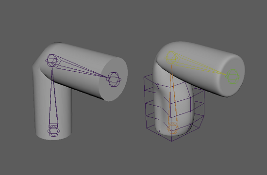
You can import both these models into a new scene (using namespaces) and use a script to extract the joint transform and the displacement between these two models in a CSV file. The full script is available in the resources for this article, but I’ll go over the important stuff here. The first thing we do is import the packages we’ll use, then we set some global parameters.

import pymel.core as pmc
import numpy as np
from random import random
# Global vars (customize before running)
linSkin_mesh_name = 'linSkin:pCylinder1'      
# name for the base model with linear skinning
linSkin_joint_name = 'linSkin:joint2'         
# model inputcustomDef_mesh_name = 'customDef:pCylinder1'  
# name for the deformed model to be approximated
customDef_joint_name = 'customDef:joint2'     
# model inputsamples = 30                                  
# samples to be collectedcsvIn = 'c:/yourPath/inputs.csv'
csvOut = 'c:/yourPath/outputs.csv'

I think most of the code above is self-explanatory. One thing I’d like to comment is about how we are sampling the data. We’ll create random transforms for the joint. The variable ‘samples’ refer to how many of these random transforms, and corresponding deformations, we’ll create.

After that, we define a function to extract the displacement amongst two meshes. Note that we construct one big list with all displacements for all mesh vertices (1).

def getMeshDisplacement(meshA, meshB):
    '''Get displacement between two Maya polygon meshes as a single row vector.'''
    # Check if meshes match
    nverts = len(meshA.verts)
    if nverts != len(meshB.verts):
        raise Exception('Meshes must have the same number of vertices.')
    # Iterate vertices and calculate displacement
    dsplc = [None]*nverts*3 # Reserve space for displacement vector
    for i in range(nverts):
        dVec3 = meshB.verts[i].getPosition() - meshA.verts[i].getPosition()
        dsplc[i*3:i*3+3] = [dVec3.x, dVec3.y, dVec3.z]
    return dsplc

Finally, in the main execution, we get the meshes and joints and generate random transforms for which we’ll sample the inputs and outputs to our model. Both transforms and displacements are stored in NDArrays so they can be easily exported as CSVs.

# Get meshes and joints
linSkin_mesh = pmc.ls(linSkin_mesh_name)[0]
linSkin_joint = pmc.ls(linSkin_joint_name)[0]
customDef_mesh = pmc.ls(customDef_mesh_name)[0]
customDef_joint = pmc.ls(customDef_joint_name)[0]
Iterate meshes over time to sample displacementsxfos = []
dsplcs = []
for i in range(samples):
    # Create a matrix with a random orientation
    randXfo = linSkin_joint.getTransformation()
    randXfo.setRotationQuaternion(randQuatDim(), randQuatDim(), randQuatDim(), randQuatDim())
    # Set transformation in both joints
    linSkin_joint.setTransformation(randXfo)
    customDef_joint.setTransformation(randXfo)
    # Joints have limitations, so one must get its actual transformation
    xfo = np.array(customDef_joint.getTransformation()).flatten() # and cast to NDArray
    # Get displacement amongst meshes
    dsplc = np.array(getMeshDisplacement(linSkin_mesh, customDef_mesh)) # and cast to NDArray
    xfos.append(xfo)
    dsplcs.append(dsplc)
    print('Built sample ' + str(i))

# Output displacement samples as CSV
xfos = np.stack(xfos)
dsplcs = np.stack(dsplcs)
np.savetxt(csvIn, xfos)
np.savetxt(csvOut, dsplcs)

There are two important things to note about the joint transformation. The first is that randQuatDim()is generating random values from -1 to 1 for every dimension in the quaternion we build. The second is that we need to get the transformation from the joints after we have set them because they have joint limitations turned on. Hence, the final transform we’ll be different than that random matrix we have created.

We limit the joint’s movement, so we won’t create random orientations that do not make sense

You can inspect the CSV files in Excel, Google Spreadsheets, or other tools of your choosing.

Train a regression Neural Network to correlate transforms to deformation

Now that you have the dataset it is time to train the network. In the resources for this post, you’ll see I have created a well-documented IPython notebook for you to run in Google Colaboratory. I’ll comment on the most critical aspects of that code here.

To train the network we’ll be using Keras, the same framework I have used in my first tutorial (here). These are all the packages you’ll need to load:

import numpy as np
import keras
from keras.models import Sequential      # An object we need to define our model
from keras.layers import Dense           # This is the type of network
from keras import utils                  # Tools to process our data
import numpy as np                       # Types for structuring our data
import matplotlib.pyplot as plt
from google.colab import files           # Input and output files from GClab

The last one (google.colab) is only relevant if you are using Google Colaboratory. If you are you might be wondering how to get your custom dataset up to that system. Here is what you’ll do:

# Upload the files you have extracted in Maya
inputs_file = files.upload()
outputs_file = files.upload()

You’ll be prompted to choose the files from your hard drive. The path to the files is stored as a key in a dict; this is how you retrieve the path and load the CSV as a Numpy NDArray:

# Get inputs and outputs from uploaded files
inputs = np.loadtxt(list(inputs_file.keys())[0])
outputs = np.loadtxt(list(outputs_file.keys())[0])

Feature Normalization

In this prototype, I’m normalizing the dataset before proceeding with the training. This step is not mandatory, and I have not done it in previous tutorials for the sake of simplicity. But it is a common practice that you should get used to because it improves the accuracy of your model at no extra cost.

The idea behind feature normalization is that some features in your dataset might be huge scalar values that vary a lot, while others might be near constant, near zero values. Such different values will have a very different impact on the activation of your neurons and will bias the network. Therefore, it is good to rescale the data to avoid such effect.

Here I’m using a widespread scaling approach, I remove the feature’s mean and divide the remainder by its standard deviation. Notice these are not the mean and standard deviation of the whole dataset, but of all samples for each feature (i.e., every component of the transform matrix, and every dimension of every displacement vector).

I create one function to normalize and another to ‘denormalize’ features:

# Implement feature normalization and denormalization functions.
def featNorm(features):    
    '''Normalize features by mean and standard deviation.    
    Returns tuple (normalizedFeatures, mean, standardDeviation).    
    ''' 
    
    mean = np.mean(features, axis=0) 
    std = np.std(features - mean, axis=0)    
    feats_norm = (features - mean) / (std + np.finfo(np.float32).eps)    
    
    return (feats_norm, mean, std)
    
def featDenorm(features_norm, mean, std):    
    '''Denormalize features by mean and standard deviation'''    
    features = (features_norm * std) + mean    
    
    return features

Note that in the ‘featNorm’ function we output not only the normalized features but the means and standard deviations. I do that because we’ll need this information to transform new data in the prediction phase, and also to ‘denormalize’ the network’s output. We apply the normalization and store the values using the following code:

inputNormalization = featNorm(inputs)
inputs_norm = inputNormalization[0]
inputs_mean = inputNormalization[1]
inputs_std = inputNormalization[2]
outputNormalization = featNorm(outputs)
outputs_norm = outputNormalization[0]
outputs_mean = outputNormalization[1]
outputs_std = outputNormalization[2]

Now that we have prepared the data, let’s train the model.

Defining the model

We represent the model using Keras sequential interface, much like we have done in the previous tutorial. The main difference is that here we are not training a classification model, but a regression model (see the video for further clarification). So, the activation function in the final layer is just a linear mapping of the activation values. Also, the loss function, the thing we are trying to minimize, is the ‘mean squared error’, that is, the squared distance between the predictions and the actual values.

We have used the number of neurons and the activation functions suggested by the authors in the paper. Although the model will work with other configurations.

model = Sequential()
model.add(Dense(512, input_dim=inputs_norm.shape[1], activation='tanh'))
model.add(Dense(512, input_dim=100, activation='tanh'))
model.add(Dense(outputs_norm.shape[1], activation='linear'))
adam = keras.optimizers.Adam(lr=0.01)
model.compile(loss='mse', optimizer=adam, metrics=['mse'])

We train the model and save the information in a history variable so that we can plot the learning graph afterward. We are reserving 30% of samples for testing (validation_split).

history = model.fit(inputs_norm, outputs_norm, epochs=200, validation_split=0.3, batch_size=None)

During training, you should see the error in the validation and training sets diminish continually. Here is the plot for my training:

Plot of a downwards slope

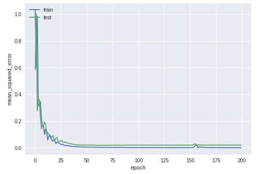
Loss (mse) diminishes along the training

After the training has finished, you can save and download your model. Remember you also need to keep the normalization data to apply it to new data during prediction:

model.save('FDDA.h5')
np.savetxt('in_mean.csv', inputs_mean)
np.savetxt('in_std.csv', inputs_std)
np.savetxt('out_mean.csv', outputs_mean)
np.savetxt('out_std.csv', outputs_std)
files.download('FDDA.h5')
files.download('in_mean.csv')
files.download('in_std.csv')
files.download('out_mean.csv')
files.download('out_std.csv')

Implement a custom deformer using the trained model

This final step is similar to what I have shown you in a previous tutorial. That is, we’ll be implementing a custom Python DG node to run our model live in Maya. But in this case, we are implementing a deformer, and Maya has a custom class for deformer nodes called MPxGeometryFilter. You should use it over MPxNode for convenience and performance. On the downside, this class is not available through OpenMaya 2, so you’ll have to stick to the old OpenMaya API. Here are the packages you’ll need to load:

import maya.OpenMayaMPx as ompx
import maya.OpenMaya as om
import numpy as np
from keras.models 
import load_model

This Python DG node has significantly more lines of code than the last example, so I took the liberty of hardcoding some things. If you don’t want to do that, make sure you check the previous tutorial.

# Declare global node params and other global vars
nodeName = 'tdl_FDDA'
nodeTypeID = om.MTypeId(0x1C3B1234)
model = load_model('c:/yourPath/dfDef.h5')
inputs_mean = np.loadtxt('c:/yourPath/in_mean.csv')
inputs_std = np.loadtxt('c:/yourPath/in_std.csv')
outputs_mean = np.loadtxt('c:/yourPath/out_mean.csv')
outputs_std = np.loadtxt('c:/yourPath/out_std.csv')

Then we implement our normalization functions once again:

# Implement feture normalization and denormalization functions.
def featNorm(features, mean, std):    
    '''Normalize features by given mean and standard deviations.'''    
    feats_norm = (features - mean) / (std + np.finfo(np.float32).eps)    
    return feats_norm
    
def featDenorm(features_norm, mean, std):
    '''Denormalize features by mean and standard deviation.'''    
    features = (features_norm * std) + mean    
    return features

Note that here the ‘featNorm’ function does not generate the ‘mean’ and ‘std’ variables but instead receives them as input parameters.

Init the node and create attributes

As you have seen in the previous tutorial the first step in creating a custom Python DG node is setting up its attributes. In this case, since we are instantiating the MPxGeometryFilter class, some attributes are given, these are the input-output geometry, and the envelope. The envelope is a multiplier of the deformation effect.

We will add one other attribute, the matrix which we’ll use as input for the Neural Network. Declare it in the init function like this:

def init():    
    # (1) Setup input attributes    
    mAttr = om.MFnMatrixAttribute()    
    tdl_FDDANode.xfoMat = mAttr.create('matrix', 'xm')    
    mAttr.writable = True    mAttr.storable = True    
    mAttr.connectable = True    mAttr.hidden = False    
    
    # (2) Add the output attributes to the node    
    # The only ouput attribute is the deformed geometry    
    # which is the default for any deformer. Hence we add    
    # no additional outputs.    
    
    # (3) Add the attributes to the node    
    tdl_FDDANode.addAttribute(tdl_FDDANode.xfoMat)    
    
    # (4) Declare attribute dependencies    
    tdl_FDDANode.attributeAffects(tdl_FDDANode.xfoMat, ompx.cvar.MPxGeometryFilter_outputGeom)

Note that in the last line we tell Maya to update the output geometry when the matrix changes the value.

Compute deformation

In the MPxGeometryFilter nodes, you do not declare a ‘compute’ function but a ‘deform’ function. The deform function provides an iterator (geom_it) that can be used to iterate over all vertices. We start the deformation by setting up all the attributes we’ll need and check if the number of vertices in the mesh matches the number of output neurons in our network.

def deform(self, data, geom_it, local_to_world_mat, geom_idx):
    # Get the default deformer's class default attributes            
    # Get mesh        
    input_attr = ompx.cvar.MPxGeometryFilter_input        
    input_geom_attr = ompx.cvar.MPxGeometryFilter_inputGeom        
    input_handle = data.outputArrayValue(input_attr)        
    input_handle.jumpToElement(geom_idx)        
    input_geom_obj = input_handle.outputValue().child(input_geom_attr).asMesh()        
    mesh = om.MFnMesh(input_geom_obj)            
    
    # Get envelope        
    envelope_attr = ompx.cvar.MPxGeometryFilter_envelope        
    envelope = data.inputValue(envelope_attr).asFloat()        
    
    # Get custom deformer attributes        
    xfoMat_handle = data.inputValue(tdl_FDDANode.xfoMat)        
    xfoMat = xfoMat_handle.asMatrix()        
    xfo = [np.float32(xfoMat(r, c)) for r in xrange(4) for c in xrange(4)]        
    
    # Check if number of vertices match the trained model        
    if (mesh.numVertices() != model.output_shape[1]/3):            
        raise Exception('Mesh has ' + str(mesh.numVertices()) + ' vertices, '
                        'model expects ' + str(model.output_shape[1] / 3) + ' vertices.')

Then we get and cache the model’s prediction, so that if the joint’s transformation does not change we don’t re-evaluate it. Note that we normalize the network’s inputs (xfo) and denormalize its outputs (prediction/displacement).

# Get and cache displacement prediction        
if (self.xfo_cache == xfo):            
    pass        
else:            
    self.xfo_cache = xfo            

# Model predictions            
xfo = np.array(xfo)            
xfo = featNorm(xfo.reshape((1, 16)), inputs_mean, inputs_std)            
prediction = featDenorm(model.predict(xfo), outputs_mean, outputs_std)            
self.prediction_cache = prediction.flatten()

Finally, we trigger the geometry iterator and update the position for every vertex. We have to get the correct x,y, and z values for every vertex and make them regular floats as the network’s outputs are Numpy.floats. Then we compose an MVector that we’ll add to the vertex position.

# Deform vertex        
while not geom_it.isDone():            
    idx = geom_it.index()            
    pos = geom_it.position()            
    # Get displacement from cached prediction            
    x = float(self.prediction_cache[idx * 3])            
    y = float(self.prediction_cache[idx * 3 + 1])            
    z = float(self.prediction_cache[idx * 3 + 2])            
    dsplc = om.MVector(x, y, z)            
    
    # Apply deformation            
    new_pos = pos + (dsplc*envelope)            
    geom_it.setPosition(new_pos)            
    geom_it.next()

Connecting everything up

If you have set everything up properly, and if your ‘3DL_FDDA.py’ file is being loaded by Maya.env (if you don’t know how to do that look up the Python DG node tutorial) you can create your new deformer using maya.cmds.

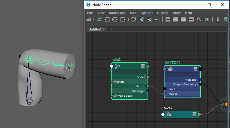
Load that base model ‘linSkin.ma’ once again, select the mesh to be deformed and run the following code from the Maya Python script editor:

import maya.cmds as cmds
cmds.deformer(type=’tdl_FDDA’)

A deformer will be created and connected to the geometry, now plug Joint2’s matrix to the deformer and voila. You should see the magic.

Custom implementation of the FDDA deformer running inside Autodesk Maya

If you have followed this tutorial up to here, congratulations, you have understood and implemented your first SIGGRAPH deep learning paper. ‘Fast and Deep Deformation Approximations’ provides an interesting solution to make character deformations faster and portable. This is a Python prototype implementation, so rest assured it won’t be fast, but all the pieces are there. The deformations look very much like the original and the model generalizes well (try to play around with the joint). While the paper is limited to movement from joint transformations I think you can see that it is not impossible to connect other things to the input and test how the model reacts.

Three cilinders bending with different kinds of deformations

Tell me what you think about this prototype. Were you able to run it properly? Can you think of similar applications that can be dealt with a model like this?