Implement a Substance like Normal Map Generator with a Convolutional Network

In this article, you’ll learn how to train a convolutional neural network to generate normal maps from color images.

Convolutional neural networks are great at dealing with images, as well as other types of structured data. If you want to understand how they work, please read this other article first.

Picture of coins and normal maps corresponding to that picture

Here is what you’ll learn in this article:

1. Data and tooling

2. Loading and pre-processing images

3. Creating and training a generative convolutional neural network

4. Visualizing results

Data and tooling

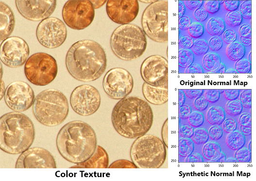
We are setting out to teach a neural network to generate normal maps from color images. We are going to do this in a ‘pair-wise’ fashion. That means we’ll show the network pairs of corresponding images, in this case, color images and normal maps. I’ll be using datasets Pixar 128 and 130, both containing Pixar textures back from 1993.

I have done some pre-processing of those two datasets to remove alpha channels and rescale the images to 256×256 pixels. This will help us do a little less pre-processing in Python. I have also organized the textures into color, and normal folders, so they are easy to load in our code. This pre-processed dataset can be downloaded in the resources for this article.

Up until now, I have been advocating the use of Google Colab for you to train your networks. Colab is ok when dealing with small datasets and easy to train topologies, but as data get bigger and topologies more complex you are better of training nets in your machine, preferably using a Nvidia GPU with decent amounts of memory.

You can always run the code in bare Python, but if you want a more elegant interface, akin to what you have in Google Colab, you can install Jupyter Notebook in your computer. I highly recommend it. Notebooks make it easy to visualize data and comment code. I suggest you install it in a regular Python install (not mayapy.exe) so you don’t need to address binary compatibility problems. You can always save your models and load them in Mayapy once trained.

Installing Jupyter is as easy as:

pip install jupyter

Running Jupyter is as easy as:

jupyter notebook(if you have Python\Scripts in your PATH environment variable)

Other libraries we’ll be using in this tutorial: Keras (with the back-end of your choice), Numpy, Matplotlib, Scikit-Image, and PyThreeJS. Make sure you have all of them installed.

All the code shown here is available as a Jupyter Notebook you can download in the resources for this article. I’ll go over the most essential bits though.

First, we load the images

data_dir = '../data/pixar/'
color_imgs = skimage.io.ImageCollection(data_dir + '/color/*.tif')
normal_imgs = skimage.io.ImageCollection(data_dir + '/normal/*.tif')

Then we make them float. Remember, these are old 8-bit and 16-bit textures.

color_imgs = skimage.img_as_float([color_imgs[x] for x in range(len(color_imgs))])
normal_imgs = skimage.img_as_float([normal_imgs[x] for x in range(len(normal_imgs))])

All images are 256×256. A convolutional network for such image size may be too big for your graphics card (2GB or less). In that case, you might want to down-res your images a bit. I have left some code in the notebook for you to do so.

The last step in this phase is to split the dataset into train and test sets. We do this to make sure we’ll only test the performance of the network on samples that it has not seen during training (or else we would be cheating). We randomize color_imgs and normal_imgs with a single random seed like this:

seed = np.random.randint(999)
np.random.seed(seed)
np.random.shuffle(color_imgs)
np.random.seed(seed)
np.random.shuffle(normal_imgs)

Then we split the first 70% and the last 30% of each of the sets into the train and test sets. It is good to check if everything is working by plotting inputs and outputs of either the train set, the test set, or both. You can use Scikit-image and Matplotlib for that.

skimage.io.imshow(skimage.img_as_ubyte(color_train_set[0]))
plt.show()

skimage.io.imshow(skimage.img_as_ubyte(normal_train_set[0]))
plt.show()

Creating and training a generative convolutional neural network

Ok, now let’s define our model. We’ll be using the Keras Model API. Let’s import everything we’ll need.

from keras.models 
import Modelfrom keras.layers 
import Input, Conv2D, AveragePooling2D, UpSampling2D, BatchNormalization
from keras.optimizers import Adam

Conv2D, as you might have guessed, is the convolutional layer. It is 2D because convolutions can happen in other dimensional spaces like 1D, and 3D.

AveragePooling2D is the type of pooling we’ll be using to down-res our feature maps (if this does not make sense to you, read this).

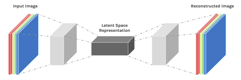
The network we’ll be building has a symmetric topology, much like an autoencoder (if you don’t know what an autoencoder is, read this). We’ll convolute our color image into a latent-space and deconvolute a normal map out of it. That is why we import UpSampling2D. It does the opposite of the pooling operation.

5 blocks representing a convolutional autoencoder

We also import BatchNormalization; a proven way to enhance convergence by normalizing the activations in each layer of the neural network. And finally, we load Adam as our optimizer.

Here is how we define our model:

input_img = Input(shape=(img_size, img_size, 3))
ng = Conv2D(15, (3, 3), activation='relu', padding='same', use_bias=False)(input_img)ng = BatchNormalization()(ng)ng = AveragePooling2D((4, 4), padding='same')(ng)ng = Conv2D(30, (3, 3), activation='relu', padding='same', use_bias=False)(ng)ng = BatchNormalization()(ng)ng = UpSampling2D((4, 4))(ng)ng = Conv2D(15, (3, 3), activation='relu', padding='same', use_bias=False)(ng)ng = BatchNormalization()(ng)ng = Conv2D(3, (3, 3), activation='sigmoid', padding='same')(ng)normal_generator = Model(input_img, ng)normal_generator.compile(Adam(amsgrad=True), loss='mse')

Note that our Conv2D layers have windows of size 3×3. Larger windows may provide better results but use more memory. The same goes for the number of filters. Talking about filters, we increase the number of filters as we reduce the feature map dimensionality, this is a common practice in defining convolutional models.

Also worthy of note is the padding, set to ‘same’. When we do this, Keras will pad the image enough so that the convolution won’t reduce its size. This is important to keep the size of the output image equal to the size of the input image.

We remove the bias of all layers that precede BatchNormalization. The biases in any neural network layer serve the purpose of rescaling the values of activations; the BatchNormalization operation does something similar by normalizing activations, so there is no need to keep both methods on. Note that we don’t normalize the last layer, where we also use sigmoid activation instead of ReLU; this is because we want to enforce pixel values between 0 and 1.

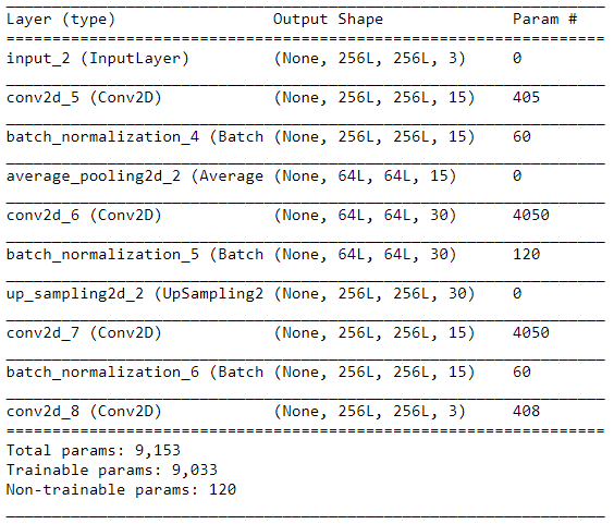
If you want to ‘see’ the network’s topology you can call normal_generator.summary(). You should get something like this:

Keras model summary with layers and the number of parameters (neurons) for each layer

We train the network using the fit function:

normal_generator.fit(color_train_set, normal_train_set,
                     validation_data = (color_test_set, normal_test_set),
                                        batch_size=batch_size,
                                        epochs=100)

To better visualize the progress of the network’s training I’ve created this function:

def test_net_with_random_image():
    idx = int(np.random.rand(1)*len(color_test_set))    
    y_legit = skimage.img_as_float(normal_test_set[idx]).reshape(1,img_size,img_size,3)    
    y_fake = generator.predict(skimage.img_as_float(color_test_set[idx]).reshape(1,img_size,img_size,3))    
    skimage.io.imshow(skimage.img_as_ubyte(y_legit).reshape(img_size,img_size,3))    
    plt.show()    
    
    skimage.io.imshow(skimage.img_as_ubyte(y_fake).reshape(img_size,img_size,3))    
    plt.show()

By using it, we can compare a real normal map to the output of the network given the corresponding color image. As you would expect, a randomly initiated and untrained network provides a highly entropic result:

One normal map and one grey box

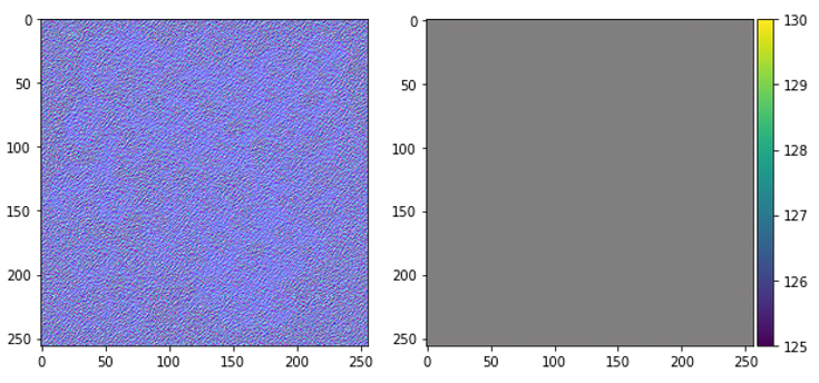
But after training it for 200 epochs, this is what you get when you call the test function again:

Two normal maps, one real and the other synthetic

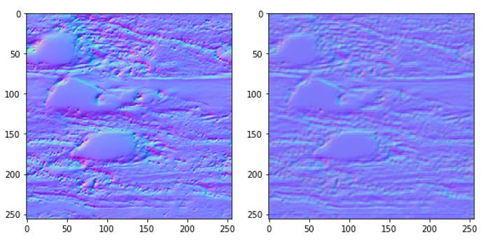
Quite impressive!

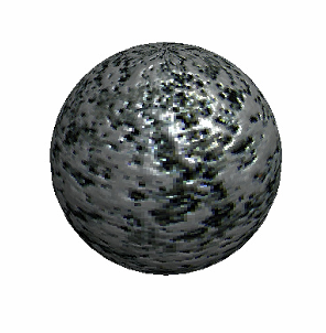
Another way to visualize the results is using PyThreeJS. You might know ThreeJS, the WebGL framework. PyThreeJS is a package that lets you call ThreeJS and use it in your Jupyter Notebook, which is excellent for rapidly visualizing 3D stuff.

Using PyThreeJS we can load a color image and a synthetic normal map to textures we can then use in any material we’d like. The textures can be declared directly from the Numpy arrays we regularly use by creating a DataTexture object and passing the Numpy array as ‘data’.

idx = int(np.random.rand(1)*len(color_test_set))
x = color_test_set[idx]
y = normal_generator.predict(skimage.img_as_float(color_test_set[idx]).reshape(1,img_size,img_size,3)).reshape(img_size,img_size,3)
color_tex = DataTexture(data=x, format="RGBFormat", type="FloatType",)
normal_tex = DataTexture(data=y, format="RGBFormat", type="FloatType",)

We then create a ball with a simple material, a camera, and a light. For the full implementation of the PyThreeJS example, please check the resources.

A CG render sphere

In conclusion

In this tutorial, you have learned how to create a convolutional neural network capable of doing pair-wise image translation. In doing so, you have learned how to create and connect convolution layers in Keras, and how to visualize 2D data with Scikit-image and 3D data with PyThreeJS.

These skills are fundamental for building and testing many other neural network topologies for different sorts of applications. Convolutional networks can be used for time-series, 3d voxels, and geometry. PyThreeJS can be used to visualize primitives, explicit meshes, and articulated figures. We are building a solid foundation to tackle more exciting models shortly.