Graphs in Python

Origins of Graph Theory

7 bridges of Koenigsberg

Before we start with the actual implementations of graphs in Python and before we start with the introduction of Python modules dealing with graphs, we want to devote ourselves to the origins of graph theory. The origins take us back in time to the Künigsberg of the 18th century. Königsberg was a city in Prussia that time. The river Pregel flowed through the town, creating two islands. The city and the islands were connected by seven bridges as shown. The inhabitants of the city were moved by the question, if it was possible to take a walk through the town by visiting each area of the town and crossing each bridge only once? Every bridge must have been crossed completely, i.e. it is not allowed to walk halfway onto a bridge and then turn around and later cross the other half from the other side. The walk need not start and end at the same spot. Leonhard Euler solved the problem in 1735 by proving that it is not possible. He found out that the choice of a route inside each land area is irrelevant and that the only thing which mattered is the order (or the sequence) in which the bridges are crossed. He had formulated an abstraction of the problem, eliminating unnecessary facts and focussing on the land areas and the bridges connecting them. This way, he created the foundations of graph theory. If we see a "land area" as a vertex and each bridge as an edge, we have "reduced" the problem to a graph.

Introduction into Graph Theory Using Python

Simple Graph with an isolated node

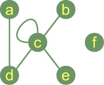
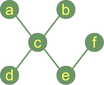
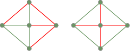
Before we start our treatise on possible Python representations of graphs, we want to present some general definitions of graphs and it's components. A "graph"1 in mathematics and computer science consists of "nodes", also known as "vertices". Nodes may or may not be connected with one another. In our illustration, - which is a pictorial representation of a graph, - the node "a" is connected with the node "c", but "a" is not connected with "b". The connecting line between two nodes is called an edge. If the edges between the nodes are undirected, the graph is called an undirected graph. If an edge is directed from one vertex (node) to another, a graph is called a directed graph. A directed edge is called an arc. Though graphs may look very theoretical, many practical problems can be represented by graphs. They are often used to model problems or situations in physics, biology, psychology and above all in computer science. In computer science, graphs are used to represent networks of communication, data organization, computational devices, the flow of computation, In the latter case, the are used to represent the data organisation, like the file system of an operating system, or communication networks. The link structure of websites can be seen as a graph as well, i.e. a directed graph, because a link is a directed edge or an arc. Python has no built-in data type or class for graphs, but it is easy to implement them in Python. One data type is ideal for representing graphs in Python, i.e. dictionaries. The graph in our illustration can be implemented in the following way:

graph = { "a" : ["c"],
          "b" : ["c", "e"],
          "c" : ["a", "b", "d", "e"],
          "d" : ["c"],
          "e" : ["c", "b"],
          "f" : []
        }

The keys of the dictionary above are the nodes of our graph. The corresponding values are lists with the nodes, which are connecting by an edge. There is no simpler and more elegant way to represent a graph. An edge can be seen as a 2-tuple with nodes as elements, i.e. ("a", "b") Function to generate the list of all edges:

def generate_edges(graph):
    edges = []
    for node in graph:
        for neighbour in graph[node]:
            edges.append((node, neighbour))

    return edges

print(generate_edges(graph))

This code generates the following output, if combined with the previously defined graph dictionary:

$ python3 graph_simple.py 
[('a', 'c'), ('c', 'a'), ('c', 'b'), ('c', 'd'), ('c', 'e'), ('b', 'c'), ('b', 'e'), ('e', 'c'), ('e', 'b'), ('d', 'c')]

As we can see, there is no edge containing the node "f". "f" is an isolated node of our graph. The following Python function calculates the isolated nodes of a given graph:

def find_isolated_nodes(graph):
    """ returns a list of isolated nodes. """
    isolated = []
    for node in graph:
        if not graph[node]:
            isolated += node
    return isolated

If we call this function with our graph, a list containing "f" will be returned: ["f"]

Graphs as a Python Class

Before we go on with writing functions for graphs, we have a first go at a Python graph class implementation. If you look at the following listing of our class, you can see in the __init__-method that we use a dictionary "self.__graph_dict" for storing the vertices and their corresponding adjacent vertices.

""" A Python Class
A simple Python graph class, demonstrating the essential 
facts and functionalities of graphs.
"""


class Graph(object):

    def __init__(self, graph_dict=None):
        """ initializes a graph object 
            If no dictionary or None is given, 
            an empty dictionary will be used
        """
        if graph_dict == None:
            graph_dict = {}
        self.__graph_dict = graph_dict

    def vertices(self):
        """ returns the vertices of a graph """
        return list(self.__graph_dict.keys())

    def edges(self):
        """ returns the edges of a graph """
        return self.__generate_edges()

    def add_vertex(self, vertex):
        """ If the vertex "vertex" is not in 
            self.__graph_dict, a key "vertex" with an empty
            list as a value is added to the dictionary. 
            Otherwise nothing has to be done. 
        """
        if vertex not in self.__graph_dict:
            self.__graph_dict[vertex] = []

    def add_edge(self, edge):
        """ assumes that edge is of type set, tuple or list; 
            between two vertices can be multiple edges! 
        """
        edge = set(edge)
        (vertex1, vertex2) = tuple(edge)
        if vertex1 in self.__graph_dict:
            self.__graph_dict[vertex1].append(vertex2)
        else:
            self.__graph_dict[vertex1] = [vertex2]

    def __generate_edges(self):
        """ A static method generating the edges of the 
            graph "graph". Edges are represented as sets 
            with one (a loop back to the vertex) or two 
            vertices 
        """
        edges = []
        for vertex in self.__graph_dict:
            for neighbour in self.__graph_dict[vertex]:
                if {neighbour, vertex} not in edges:
                    edges.append({vertex, neighbour})
        return edges

    def __str__(self):
        res = "vertices: "
        for k in self.__graph_dict:
            res += str(k) + " "
        res += "\nedges: "
        for edge in self.__generate_edges():
            res += str(edge) + " "
        return res


if __name__ == "__main__":

    g = { "a" : ["d"],
          "b" : ["c"],
          "c" : ["b", "c", "d", "e"],
          "d" : ["a", "c"],
          "e" : ["c"],
          "f" : []
        }


    graph = Graph(g)

    print("Vertices of graph:")
    print(graph.vertices())

    print("Edges of graph:")
    print(graph.edges())

    print("Add vertex:")
    graph.add_vertex("z")

    print("Vertices of graph:")
    print(graph.vertices())
 
    print("Add an edge:")
    graph.add_edge({"a","z"})
    
    print("Vertices of graph:")
    print(graph.vertices())

    print("Edges of graph:")
    print(graph.edges())

    print('Adding an edge {"x","y"} with new vertices:')
    graph.add_edge({"x","y"})
    print("Vertices of graph:")
    print(graph.vertices())
    print("Edges of graph:")
    print(graph.edges())
  

If you start this module standalone, you will get the following result:

$ python3 graph.py 
Vertices of graph:
['a', 'c', 'b', 'e', 'd', 'f']
Edges of graph:
[{'a', 'd'}, {'c', 'b'}, {'c'}, {'c', 'd'}, {'c', 'e'}]
Add vertex:
Vertices of graph:
['a', 'c', 'b', 'e', 'd', 'f', 'z']
Add an edge:
Vertices of graph:
['a', 'c', 'b', 'e', 'd', 'f', 'z']
Edges of graph:
[{'a', 'd'}, {'c', 'b'}, {'c'}, {'c', 'd'}, {'c', 'e'}, {'a', 'z'}]
Adding an edge {"x","y"} with new vertices:
Vertices of graph:
['a', 'c', 'b', 'e', 'd', 'f', 'y', 'z']
Edges of graph:
[{'a', 'd'}, {'c', 'b'}, {'c'}, {'c', 'd'}, {'c', 'e'}, {'a', 'z'}, {'y', 'x'}]

Paths in Graphs

We want to find now the shortest path from one node to another node. Before we come to the Python code for this problem, we will have to present some formal definitions. Adjacent vertices: Two vertices are adjacent when they are both incident to a common edge. Path in an undirected Graph: A path in an undirected graph is a sequence of vertices $P = ( v_1, v_2, ..., v_n ) ∈ V x V x ... x V$ such that vi is adjacent to $v_{i+1}$ for $1 ≤ i < n$. Such a path $P$ is called a path of length $n$ from $v_1$ to $v_n$.

Simple Path: A path with no repeated vertices is called a simple path. Example: (a, c, e) is a simple path in our graph, as well as (a, c, e, b). (a, c, e, b, c, d) is a path but not a simple path, because the node c appears twice. The following method finds a path from a start vertex to an end vertex:

    def find_path(self, start_vertex, end_vertex, path=None):
        """ find a path from start_vertex to end_vertex 
            in graph """
        if path == None:
            path = []
        graph = self.__graph_dict
        path = path + [start_vertex]
        if start_vertex == end_vertex:
            return path
        if start_vertex not in graph:
            return None
        for vertex in graph[start_vertex]:
            if vertex not in path:
                extended_path = self.find_path(vertex, 
                                               end_vertex, 
                                               path)
                if extended_path: 
                    return extended_path
        return None

If we save our graph class including the find_path method as "graphs.py", we can check the way of working of our find_path function:

from graphs import Graph

g = { "a" : ["d"],
      "b" : ["c"],
      "c" : ["b", "c", "d", "e"],
      "d" : ["a", "c"],
      "e" : ["c"],
      "f" : []
    }


graph = Graph(g)

print("Vertices of graph:")
print(graph.vertices())

print("Edges of graph:")
print(graph.edges())


print('The path from vertex "a" to vertex "b":')
path = graph.find_path("a", "b")
print(path)

print('The path from vertex "a" to vertex "f":')
path = graph.find_path("a", "f")
print(path)

print('The path from vertex "c" to vertex "c":')
path = graph.find_path("c", "c")
print(path)

The result of the previous program looks like this:

Vertices of graph:
['e', 'a', 'd', 'f', 'c', 'b']
Edges of graph:
[{'e', 'c'}, {'a', 'd'}, {'d', 'c'}, {'b', 'c'}, {'c'}]
The path from vertex "a" to vertex "b":
['a', 'd', 'c', 'b']
The path from vertex "a" to vertex "f":
None
The path from vertex "c" to vertex "c":
['c']

The method find_all_paths finds all the paths between a start vertex to an end vertex:

    def find_all_paths(self, start_vertex, end_vertex, path=[]):
        """ find all paths from start_vertex to 
            end_vertex in graph """
        graph = self.__graph_dict 
        path = path + [start_vertex]
        if start_vertex == end_vertex:
            return [path]
        if start_vertex not in graph:
            return []
        paths = []
        for vertex in graph[start_vertex]:
            if vertex not in path:
                extended_paths = self.find_all_paths(vertex, 
                                                     end_vertex, 
                                                     path)
                for p in extended_paths: 
                    paths.append(p)
        return paths

We slightly changed our example graph by adding edges from "a" to "f" and from "f" to "d" to test the previously defined method:

from graphs import Graph

g = { "a" : ["d", "f"],
      "b" : ["c"],
      "c" : ["b", "c", "d", "e"],
      "d" : ["a", "c"],
      "e" : ["c"],
      "f" : ["d"]
    }


graph = Graph(g)

print("Vertices of graph:")
print(graph.vertices())

print("Edges of graph:")
print(graph.edges())


print('All paths from vertex "a" to vertex "b":')
path = graph.find_all_paths("a", "b")
print(path)

print('All paths from vertex "a" to vertex "f":')
path = graph.find_all_paths("a", "f")
print(path)

print('All paths from vertex "c" to vertex "c":')
path = graph.find_all_paths("c", "c")
print(path)

The result looks like this:

Vertices of graph:
['d', 'c', 'b', 'a', 'e', 'f']
Edges of graph:
[{'d', 'a'}, {'d', 'c'}, {'c', 'b'}, {'c'}, {'c', 'e'}, {'f', 'a'}, {'d', 'f'}]
All paths from vertex "a" to vertex "b":
[['a', 'd', 'c', 'b'], ['a', 'f', 'd', 'c', 'b']]
All paths from vertex "a" to vertex "f":
[['a', 'f']]
All paths from vertex "c" to vertex "c":
[['c']]

Degree

Simple Graph with with a loop

The degree of a vertex $v$ in a graph is the number of edges connecting it, with loops counted twice. The degree of a vertex $v$ is denoted $deg(v)$. The maximum degree of a graph $G$, denoted by $Δ(G)$, and the minimum degree of a graph, denoted by $δ(G)$, are the maximum and minimum degree of its vertices. In the graph on the right side, the maximum degree is 5 at vertex $c$ and the minimum degree is 0, i.e the isolated vertex $f$. If all the degrees in a graph are the same, the graph is a regular graph. In a regular graph, all degrees are the same, and so we can speak of the degree of the graph. The degree sum formula (Handshaking lemma): $\huge ∑v ∈ Vdeg(v) = 2 |E|$ This means that the sum of degrees of all the vertices is equal to the number of edges multiplied by 2. We can conclude that the number of vertices with odd degree has to be even. This statement is known as the handshaking lemma. The name "handshaking lemma" stems from a popular mathematical problem: In any group of people the number of people who have shaken hands with an odd number of other people from the group is even. The following method calculates the degree of a vertex:

    def vertex_degree(self, vertex):
        """ The degree of a vertex is the number of edges connecting
            it, i.e. the number of adjacent vertices. Loops are counted 
            double, i.e. every occurence of vertex in the list 
            of adjacent vertices. """ 
        adj_vertices =  self.__graph_dict[vertex]
        degree = len(adj_vertices) + adj_vertices.count(vertex)
        return degree

The following method calculates a list containing the isolated vertices of a graph:

    def find_isolated_vertices(self):
        """ returns a list of isolated vertices. """
        graph = self.__graph_dict
        isolated = []
        for vertex in graph:
            print(isolated, vertex)
            if not graph[vertex]:
                isolated += [vertex]
        return isolated

The methods delta and Delta can be used to calculate the minimum and maximum degree of a vertex respectively:

    def delta(self):
        """ the minimum degree of the vertices """
        min = 100000000
        for vertex in self.__graph_dict:
            vertex_degree = self.vertex_degree(vertex)
            if vertex_degree < min:
                min = vertex_degree
        return min
        
    def Delta(self):
        """ the maximum degree of the vertices """
        max = 0
        for vertex in self.__graph_dict:
            vertex_degree = self.vertex_degree(vertex)
            if vertex_degree > max:
                max = vertex_degree
        return max

Degree Sequence

The degree sequence of an undirected graph is defined as the sequence of its vertex degrees in a non-increasing order. The following method returns a tuple with the degree sequence of the instance graph:

    def degree_sequence(self):
        """ calculates the degree sequence """
        seq = []
        for vertex in self.__graph_dict:
            seq.append(self.vertex_degree(vertex))
        seq.sort(reverse=True)
        return tuple(seq)

The degree sequence of our example graph is the following sequence of integers: (5, 2, 1, 1, 1, 0). Isomorphic graphs have the same degree sequence. However, two graphs with the same degree sequence are not necessarily isomorphic. There is the question whether a given degree sequence can be realized by a simple graph. The Erdös-Gallai theorem states that a non-increasing sequence of n numbers $d_i$ (for i = 1, ..., n) is the degree sequence of a simple graph if and only if the sum of the sequence is even and the following condition is fulfilled:

Erdös-Gallai theorem

Implementation of the Erdös-Gallai theorem

Our graph class - see further down for a complete listing - contains a method "erdoes_gallai" which decides, if a sequence fulfills the Erdös-Gallai theorem. First, we check, if the sum of the elements of the sequence is odd. If so the function returns False, because the Erdös-Gallai theorem can't be fulfilled anymore. After this we check with the static method is_degree_sequence whether the input sequence is a degree sequence, i.e. that the elements of the sequence are non-increasing. This is kind of superfluous, as the input is supposed to be a degree sequence, so you may drop this check for efficiency. Now, we check in the body of the second if statement, if the inequation of the theorem is fulfilled:

    @staticmethod
    def erdoes_gallai(dsequence):
        """ Checks if the condition of the Erdoes-Gallai inequality 
            is fullfilled 
        """
        if sum(dsequence) % 2:
            # sum of sequence is odd
            return False
        if Graph.is_degree_sequence(dsequence):
            for k in range(1,len(dsequence) + 1):
                left = sum(dsequence[:k])
                right =  k * (k-1) + sum([min(x,k) for x in dsequence[k:]])
                if left > right:
                    return False
        else:
            # sequence is increasing
            return False
        return True

Version without the superfluous degree sequence test:

    @staticmethod
    def erdoes_gallai(dsequence):
        """ Checks if the condition of the Erdoes-Gallai inequality 
            is fullfilled 
            dsequence has to be a valid degree sequence
        """
        if sum(dsequence) % 2:
            # sum of sequence is odd
            return False
        for k in range(1,len(dsequence) + 1):
            left = sum(dsequence[:k])
            right =  k * (k-1) + sum([min(x,k) for x in dsequence[k:]])
            if left > right:
                return False
        return True

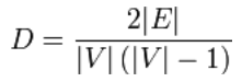
Graph Density

The graph density is defined as the ratio of the number of edges of a given graph, and the total number of edges, the graph could have. In other words: It measures how close a given graph is to a complete graph. The maximal density is 1, if a graph is complete. This is clear, because the maximum number of edges in a graph depends on the vertices and can be calculated as: $\text{max. number of edges} = ½ * |V| * ( |V| - 1 )$. On the other hand the minimal density is 0, if the graph has no edges, i.e. it is an isolated graph. For undirected simple graphs, the graph density is defined as: A dense graph is a graph in which the number of edges is close to the maximal number of edges. A graph with only a few edges, is called a sparse graph. The definition for those two terms is not very sharp, i.e. there is no least upper bound (supremum) for a sparse density and no greatest lower bound (infimum) for defining a dense graph. The precisest mathematical notation uses the big O notation: Sparse Graph: Dense Graph: A dense graph is a graph $G = (V, E)$ in which $|E| = Θ(|V|2)$. "density" is a method of our class to calculate the density of a graph:

    def density(self):
        """ method to calculate the density of a graph """
        g = self.__graph_dict
        V = len(g.keys())
        E = len(self.edges())
        return 2.0 * E / (V *(V - 1))

We can test this method with the following script.

from graph2 import Graph

g = { "a" : ["d","f"],
       "b" : ["c","b"],
       "c" : ["b", "c", "d", "e"],
       "d" : ["a", "c"],
       "e" : ["c"],
       "f" : ["a"]
}

complete_graph = { 
    "a" : ["b","c"],
    "b" : ["a","c"],
    "c" : ["a","b"]
}

isolated_graph = { 
    "a" : [],
    "b" : [],
    "c" : []
}


graph = Graph(g)
print(graph.density())

graph = Graph(complete_graph)
print(graph.density())

graph = Graph(isolated_graph)
print(graph.density())

A complete graph has a density of 1 and isolated graph has a density of 0, as we can see from the results of the previous test script:

$ python test_density.py 
0.466666666667
1.0
0.0

Connected Graphs

Connected Graph

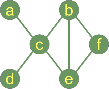
A graph is said to be connected if every pair of vertices in the graph is connected. The example graph on the right side is a connected graph. It possible to determine with a simple algorithm whether a graph is connected:

1. Choose an arbitrary node x of the graph G as the starting point

2. Determine the set A of all the nodes which can be reached from x.

3. If A is equal to the set of nodes of G, the graph is connected; otherwise it is disconnected.

We implement a method is_connected to check if a graph is a connected graph. We don't put emphasis on efficiency but on readability.

    def is_connected(self, 
                     vertices_encountered = None, 
                     start_vertex=None):
        """ determines if the graph is connected """
        if vertices_encountered is None:
            vertices_encountered = set()
        gdict = self.__graph_dict        
        vertices = list(gdict.keys()) # "list" necessary in Python 3 
        if not start_vertex:
            # chosse a vertex from graph as a starting point
            start_vertex = vertices[0]
        vertices_encountered.add(start_vertex)
        if len(vertices_encountered) != len(vertices):
            for vertex in gdict[start_vertex]:
                if vertex not in vertices_encountered:
                    if self.is_connected(vertices_encountered, vertex):
                        return True
        else:
            return True
        return False

If you add this method to our graph class, we can test it with the following script. Assuming that you save the graph class as graph2.py:

from graph2 import Graph

g = { "a" : ["d"],
      "b" : ["c"],
      "c" : ["b", "c", "d", "e"],
      "d" : ["a", "c"],
      "e" : ["c"],
      "f" : []
}

g2 = { "a" : ["d","f"],
       "b" : ["c"],
       "c" : ["b", "c", "d", "e"],
       "d" : ["a", "c"],
       "e" : ["c"],
       "f" : ["a"]
}

g3 = { "a" : ["d","f"],
       "b" : ["c","b"],
       "c" : ["b", "c", "d", "e"],
       "d" : ["a", "c"],
       "e" : ["c"],
       "f" : ["a"]
}


graph = Graph(g)
print(graph)
print(graph.is_connected())

graph = Graph(g2)
print(graph)
print(graph.is_connected())

graph = Graph(g3)
print(graph)
print(graph.is_connected())

A connected component is a maximal connected subgraph of G. Each vertex belongs to exactly one connected component, as does each edge.

Distance and Diameter of a Graph

Connected Graph showing the diameter

The distance "dist" between two vertices in a graph is the length of the shortest path between these vertices. No backtracks, detours, or loops are allowed for the calculation of a distance. In our example graph on the right, the distance between the vertex a and the vertex f is 3, i.e. dist(a,f) = 3, because the shortest way is via the vertices c and e (or c and b alternatively). The eccentricity of a vertex s of a graph g is the maximal distance to every other vertex of the graph: e(s) = max( { dist(s,v) | v ∈ V }) (V is the set of all vertices of g) The diameter d of a graph is defined as the maximum eccentricity of any vertex in the graph. This means that the diameter is the length of the shortest path between the most distanced nodes. To determine the diameter of a graph, first find the shortest path between each pair of vertices. The greatest length of any of these paths is the diameter of the graph. We can directly see in our example graph that the diameter is 3, because the minimal length between a and f is 3 and there is no other pair of vertices with a longer path. The following method implements an algorithm to calculate the diameter.

    def diameter(self):
        """ calculates the diameter of the graph """
        
        v = self.vertices() 
        pairs = [ (v[i],v[j]) for i in range(len(v)-1) for j in range(i+1, len(v))]
        smallest_paths = []
        for (s,e) in pairs:
            paths = self.find_all_paths(s,e)
            smallest = sorted(paths, key=len)[0]
            smallest_paths.append(smallest)

        smallest_paths.sort(key=len)

        # longest path is at the end of list, 
        # i.e. diameter corresponds to the length of this path
        diameter = len(smallest_paths[-1]) - 1
        return diameter

We can calculate the diameter of our example graph with the following script, assuming again, that our complete graph class is saved as graph2.py:

from graph2 import Graph

g = { "a" : ["c"],
      "b" : ["c","e","f"],
      "c" : ["a","b","d","e"],
      "d" : ["c"],
      "e" : ["b","c","f"],
      "f" : ["b","e"]
}


graph = Graph(g)

diameter = graph.diameter()

print(diameter)

It will print out the value 3.

The Complete Python Graph Class

In the following Python code, you find the complete Python Class Module with all the discussed methodes: graph2.py

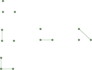
Tree / Forest

A tree is an undirected graph which contains no cycles. This means that any two vertices of the graph are connected by exactly one simple path. A forest is a disjoint union of trees. Contrary to forests in nature, a forest in graph theory can consist of a single tree! A graph with one vertex and no edge is a tree (and a forest). An example of a tree: While the previous example depicts a graph which is a tree and forest, the following picture shows a graph which consists of two trees, i.e. the graph is a forest but not a tree:

Overview of forests:

With one vertex: Forest graphs with two vertices: Forest graphs with three vertices:

Spanning Tree

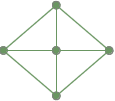
A spanning tree T of a connected, undirected graph G is a subgraph G' of G, which is a tree, and G' contains all the vertices and a subset of the edges of G. G' contains all the edges of G, if G is a tree graph. Informally, a spanning tree of G is a selection of edges of G that form a tree spanning every vertex. That is, every vertex lies in the tree, but no cycles (or loops) are contained. Example: A fully connected graph: Two spanning trees from the previous fully connected graph:

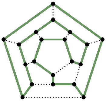
Hamiltonian Game

An Hamiltonian path is a path in an undirected or directed graph that visits each vertex exactly once. A Hamiltonian cycle (or circuit) is a Hamiltonian path that is a cycle. Note for computer scientists: Generally, it is not not possible to determine, whether such paths or cycles exist in arbitrary graphs, because the Hamiltonian path problem has been proven to be NP-complete. It is named after William Rowan Hamilton who invented the so-called "icosian game", or Hamilton's puzzle, which involves finding a Hamiltonian cycle in the edge graph of the dodecahedron. Hamilton solved this problem using the icosian calculus, an algebraic structure based on roots of unity with many similarities to the quaternions, which he also invented.

Hamilton Path, The Icosian Game

Complete Listing of the Graph Class

""" A Python Class
A simple Python graph class, demonstrating the essential 
facts and functionalities of graphs.
"""

class Graph(object):

    def __init__(self, graph_dict=None):
        """ initializes a graph object 
            If no dictionary or None is given, an empty dictionary will be used
        """
        if graph_dict == None:
            graph_dict = {}
        self.__graph_dict = graph_dict


    def vertices(self):
        """ returns the vertices of a graph """
        return list(self.__graph_dict.keys())

    def edges(self):
        """ returns the edges of a graph """
        return self.__generate_edges()

    def add_vertex(self, vertex):
        """ If the vertex "vertex" is not in 
            self.__graph_dict, a key "vertex" with an empty
            list as a value is added to the dictionary. 
            Otherwise nothing has to be done. 
        """
        if vertex not in self.__graph_dict:
            self.__graph_dict[vertex] = []

    def add_edge(self, edge):
        """ assumes that edge is of type set, tuple or list; 
            between two vertices can be multiple edges! 
        """
        edge = set(edge)
        vertex1 = edge.pop()
        if edge:
            # not a loop
            vertex2 = edge.pop()
        else:
            # a loop
            vertex2 = vertex1
        if vertex1 in self.__graph_dict:
            self.__graph_dict[vertex1].append(vertex2)
        else:
            self.__graph_dict[vertex1] = [vertex2]

    def __generate_edges(self):
        """ A static method generating the edges of the 
            graph "graph". Edges are represented as sets 
            with one (a loop back to the vertex) or two 
            vertices 
        """
        edges = []
        for vertex in self.__graph_dict:
            for neighbour in self.__graph_dict[vertex]:
                if {neighbour, vertex} not in edges:
                    edges.append({vertex, neighbour})
        return edges

    def __str__(self):
        res = "vertices: "
        for k in self.__graph_dict:
            res += str(k) + " "
        res += "\nedges: "
        for edge in self.__generate_edges():
            res += str(edge) + " "
        return res

    def find_isolated_vertices(self):
        """ returns a list of isolated vertices. """
        graph = self.__graph_dict
        isolated = []
        for vertex in graph:
            print(isolated, vertex)
            if not graph[vertex]:
                isolated += [vertex]
        return isolated

    def find_path(self, start_vertex, end_vertex, path=[]):
        """ find a path from start_vertex to end_vertex 
            in graph """
        graph = self.__graph_dict
        path = path + [start_vertex]
        if start_vertex == end_vertex:
            return path
        if start_vertex not in graph:
            return None
        for vertex in graph[start_vertex]:
            if vertex not in path:
                extended_path = self.find_path(vertex, 
                                               end_vertex, 
                                               path)
                if extended_path: 
                    return extended_path
        return None
    

    def find_all_paths(self, start_vertex, end_vertex, path=[]):
        """ find all paths from start_vertex to 
            end_vertex in graph """
        graph = self.__graph_dict 
        path = path + [start_vertex]
        if start_vertex == end_vertex:
            return [path]
        if start_vertex not in graph:
            return []
        paths = []
        for vertex in graph[start_vertex]:
            if vertex not in path:
                extended_paths = self.find_all_paths(vertex, 
                                                     end_vertex, 
                                                     path)
                for p in extended_paths: 
                    paths.append(p)
        return paths

    def is_connected(self, 
                     vertices_encountered = None, 
                     start_vertex=None):
        """ determines if the graph is connected """
        if vertices_encountered is None:
            vertices_encountered = set()
        gdict = self.__graph_dict        
        vertices = list(gdict.keys()) # "list" necessary in Python 3 
        if not start_vertex:
            # chosse a vertex from graph as a starting point
            start_vertex = vertices[0]
        vertices_encountered.add(start_vertex)
        if len(vertices_encountered) != len(vertices):
            for vertex in gdifrom graph2 import Graph

g = { "a" : ["d"],
      "b" : ["c"],
      "c" : ["b", "c", "d", "e"],
      "d" : ["a", "c"],
      "e" : ["c"],
      "f" : []
    }

graph = Graph(g)
print(graph)

for node in graph.vertices():
    print(graph.vertex_degree(node))

print("List of isolated vertices:")
print(graph.find_isolated_vertices())

print("""A path from "a" to "e":""")
print(graph.find_path("a", "e"))

print("""All pathes from "a" to "e":""")
print(graph.find_all_paths("a", "e"))

print("The maximum degree of the graph is:")
print(graph.Delta())

print("The minimum degree of the graph is:")
print(graph.delta())

print("Edges:")
print(graph.edges())

print("Degree Sequence: ")
ds = graph.degree_sequence()
print(ds)

fullfilling = [ [2, 2, 2, 2, 1, 1], 
                     [3, 3, 3, 3, 3, 3],
                     [3, 3, 2, 1, 1]
                   ] 
non_fullfilling = [ [4, 3, 2, 2, 2, 1, 1],
                    [6, 6, 5, 4, 4, 2, 1],
                    [3, 3, 3, 1] ]

for sequence in fullfilling + non_fullfilling :
    print(sequence, Graph.erdoes_gallai(sequence))

print("Add vertex 'z':")
graph.add_vertex("z")
print(graph)

print("Add edge ('x','y'): ")
graph.add_edge(('x', 'y'))
print(graph)

print("Add edge ('a','d'): ")
graph.add_edge(('a', 'd'))
print(graph)
ct[start_vertex]:
                if vertex not in vertices_encountered:
                    if self.is_connected(vertices_encountered, vertex):
                        return True
        else:
            return True
        return False

    def vertex_degree(self, vertex):
        """ The degree of a vertex is the number of edges connecting
            it, i.e. the number of adjacent vertices. Loops are counted 
            double, i.e. every occurence of vertex in the list 
            of adjacent vertices. """ 
        adj_vertices =  self.__graph_dict[vertex]
        degree = len(adj_vertices) + adj_vertices.count(vertex)
        return degree

    def degree_sequence(self):
        """ calculates the degree sequence """
        seq = []
        for vertex in self.__graph_dict:
            seq.append(self.vertex_degree(vertex))
        seq.sort(reverse=True)
        return tuple(seq)

    @staticmethod
    def is_degree_sequence(sequence):
        """ Method returns True, if the sequence "sequence" is a 
            degree sequence, i.e. a non-increasing sequence. 
            Otherwise False is returned.
        """
        # check if the sequence sequence is non-increasing:
        return all( x>=y for x, y in zip(sequence, sequence[1:]))
  

    def delta(self):
        """ the minimum degree of the vertices """
        min = 100000000
        for vertex in self.__graph_dict:
            vertex_degree = self.vertex_degree(vertex)
            if vertex_degree < min:
                min = vertex_degree
        return min
        
    def Delta(self):
        """ the maximum degree of the vertices """
        max = 0
        for vertex in self.__graph_dict:
            vertex_degree = self.vertex_degree(vertex)
            if vertex_degree > max:
                max = vertex_degree
        return max

    def density(self):
        """ method to calculate the density of a graph """
        g = self.__graph_dict
        V = len(g.keys())
        E = len(self.edges())
        return 2.0 * E / (V *(V - 1))

    def diameter(self):
        """ calculates the diameter of the graph """
        
        v = self.vertices() 
        pairs = [ (v[i],v[j]) for i in range(len(v)) for j in range(i+1, len(v)-1)]
        smallest_paths = []
        for (s,e) in pairs:
            paths = self.find_all_paths(s,e)
            smallest = sorted(paths, key=len)[0]
            smallest_paths.append(smallest)

        smallest_paths.sort(key=len)

        # longest path is at the end of list, 
        # i.e. diameter corresponds to the length of this path
        diameter = len(smallest_paths[-1]) - 1
        return diameter

    @staticmethod
    def erdoes_gallai(dsequence):
        """ Checks if the condition of the Erdoes-Gallai inequality 
            is fullfilled 
        """
        if sum(dsequence) % 2:
            # sum of sequence is odd
            return False
        if Graph.is_degree_sequence(dsequence):
            for k in range(1,len(dsequence) + 1):
                left = sum(dsequence[:k])
                right =  k * (k-1) + sum([min(x,k) for x in dsequence[k:]])
                if left > right:
                    return False
        else:
            # sequence is increasing
            return False
        return True

We can test this Graph class with the following program:

from graphs import Graph

g = { "a" : ["d"],
      "b" : ["c"],
      "c" : ["b", "c", "d", "e"],
      "d" : ["a", "c"],
      "e" : ["c"],
      "f" : []
    }

graph = Graph(g)
print(graph)

for node in graph.vertices():
    print(graph.vertex_degree(node))

print("List of isolated vertices:")
print(graph.find_isolated_vertices())

print("""A path from "a" to "e":""")
print(graph.find_path("a", "e"))

print("""All pathes from "a" to "e":""")
print(graph.find_all_paths("a", "e"))

print("The maximum degree of the graph is:")
print(graph.Delta())

print("The minimum degree of the graph is:")
print(graph.delta())

print("Edges:")
print(graph.edges())

print("Degree Sequence: ")
ds = graph.degree_sequence()
print(ds)

fullfilling = [ [2, 2, 2, 2, 1, 1], 
                     [3, 3, 3, 3, 3, 3],
                     [3, 3, 2, 1, 1]
                   ] 
non_fullfilling = [ [4, 3, 2, 2, 2, 1, 1],
                    [6, 6, 5, 4, 4, 2, 1],
                    [3, 3, 3, 1] ]

for sequence in fullfilling + non_fullfilling :
    print(sequence, Graph.erdoes_gallai(sequence))

print("Add vertex 'z':")
graph.add_vertex("z")
print(graph)

print("Add edge ('x','y'): ")
graph.add_edge(('x', 'y'))
print(graph)

print("Add edge ('a','d'): ")
graph.add_edge(('a', 'd'))
print(graph)

If we start this program, we get the following output:

vertices: c e f a d b 
edges: {'c', 'b'} {'c'} {'c', 'd'} {'c', 'e'} {'d', 'a'} 
5
1
0
1
2
1
List of isolated vertices:
[] c
[] e
[] f
['f'] a
['f'] d
['f'] b
['f']
A path from "a" to "e":
['a', 'd', 'c', 'e']
All pathes from "a" to "e":
[['a', 'd', 'c', 'e']]
The maximum degree of the graph is:
5
The minimum degree of the graph is:
0
Edges:
[{'c', 'b'}, {'c'}, {'c', 'd'}, {'c', 'e'}, {'d', 'a'}]
Degree Sequence: 
(5, 2, 1, 1, 1, 0)
[2, 2, 2, 2, 1, 1] True
[3, 3, 3, 3, 3, 3] True
[3, 3, 2, 1, 1] True
[4, 3, 2, 2, 2, 1, 1] False
[6, 6, 5, 4, 4, 2, 1] False
[3, 3, 3, 1] False
Add vertex 'z':
vertices: c e f z a d b 
edges: {'c', 'b'} {'c'} {'c', 'd'} {'c', 'e'} {'d', 'a'} 
Add edge ('x','y'): 
vertices: c e f z a y d b 
edges: {'c', 'b'} {'c'} {'c', 'd'} {'c', 'e'} {'d', 'a'} {'y', 'x'} 
Add edge ('a','d'): 
vertices: c e f z a y d b 
edges: {'c', 'b'} {'c'} {'c', 'd'} {'c', 'e'} {'d', 'a'} {'y', 'x'} 

Footnotes: 1 The graphs studied in graph theory (and in this chapter of our Python tutorial) should not be confused with the graphs of functions 2 A singleton is a set that contains exactly one element. Credits: Narayana Chikkam, nchikkam(at)gmail(dot)com, pointed out an index error in the "erdoes_gallai" method. Thank you very much, Narayana!